Matakuliah Tahun 2009 K 0442 -Metode

Matakuliah Tahun : 2009 : K 0442 -Metode Kuantitatif Simulation Pertemuan 13

Material Outline • Risk Analysis • Inventory Simulation • Waiting Line Simulation

Risk Analysis is the process of predicting the outcome of a decision in the face of uncertainty Bina Nusantara University 4

Risk Analysis Porta. Com Project Porta. Com manufactures personal computer and related equipment. Portacom’s product design group developed a prototype for a new high-quality portable printer. The New printer features an innovative design and has the potential to capture a significant share of the portable printer market Preliminary marketing and financial analysis provided the following selling price, first year administrative cost, and first-year advertising cost Selling Price = $249 per unit Administrative Cost = $400, 000 Advertising Cost = $600, 000 Bina Nusantara University …. . continued 5

Risk Analysis Porta. Com Project The cost of direct labor, the cost of part, and the first-year demand for the printer are not known with certainty and are considered probability inputs. At this stage of the planning process, Porta. Com’s best estimates of these inputs are $45 per unit for the direct labor cost, $90 per unit for the parts cost, and 15, 000 units for the first-year demand. Porta. Com would like an analysis of the first year profit potential for the printer. Because of Portacom’s tight cash flow situation, management is particularly concerned about the potential for a loss Bina Nusantara University 6

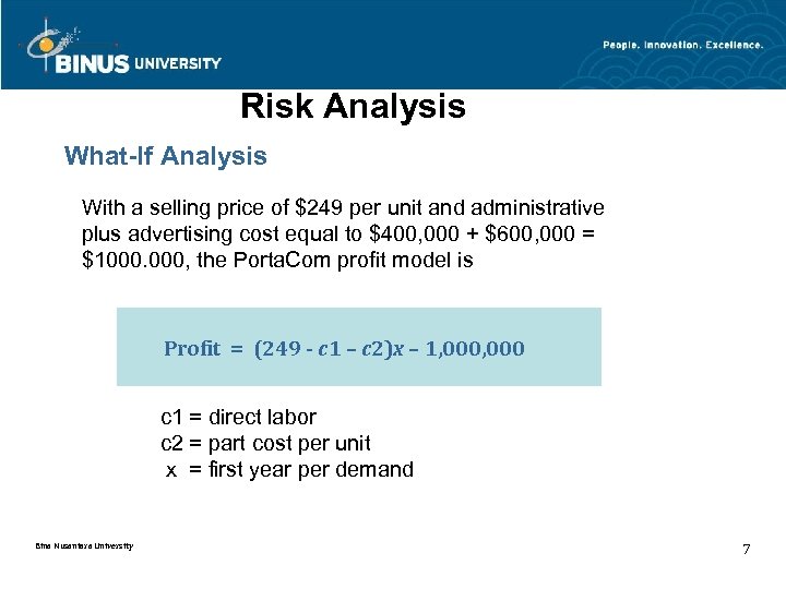Risk Analysis What-If Analysis With a selling price of $249 per unit and administrative plus advertising cost equal to $400, 000 + $600, 000 = $1000. 000, the Porta. Com profit model is Profit = (249 - c 1 – c 2)x – 1, 000 c 1 = direct labor c 2 = part cost per unit x = first year per demand Bina Nusantara University 7

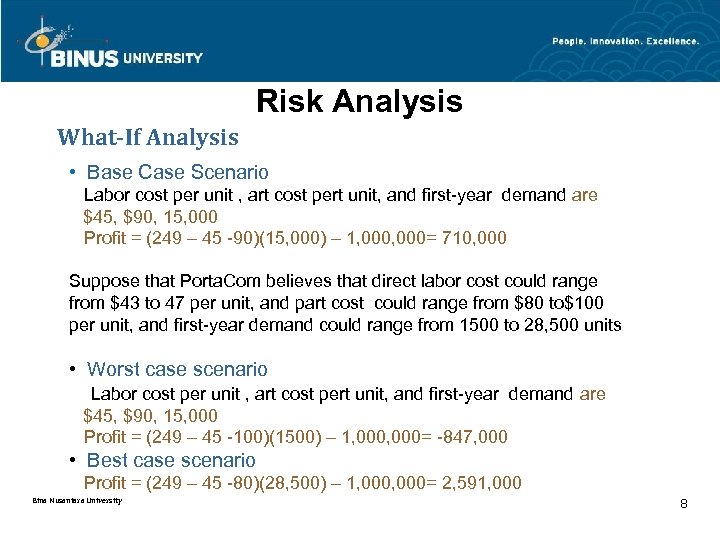Risk Analysis What-If Analysis • Base Case Scenario Labor cost per unit , art cost pert unit, and first-year demand are $45, $90, 15, 000 Profit = (249 – 45 -90)(15, 000) – 1, 000= 710, 000 Suppose that Porta. Com believes that direct labor cost could range from $43 to 47 per unit, and part cost could range from $80 to$100 per unit, and first-year demand could range from 1500 to 28, 500 units • Worst case scenario Labor cost per unit , art cost pert unit, and first-year demand are $45, $90, 15, 000 Profit = (249 – 45 -100)(1500) – 1, 000= -847, 000 • Best case scenario Profit = (249 – 45 -80)(28, 500) – 1, 000= 2, 591, 000 Bina Nusantara University 8

Inventory Simulation • Example : Butler Electrical Supply Company The product is a home ventilation fan distributed by the Butler Electrical Supply Company, Each fan costs Butler $75 and sell for$125. Thus Butler realizes a gross profit of $125 -$75 = $50 for each fan sold. Monthly demand for the fan is describe by a normal probability distribution with a mean of 100 unit and standard deviation 20 units. If monthly demand is less than the replenishment level, inventory holding cost of $15 is charged for each unit that is not sold. If monthly demand is a greater than the replenishment level, a stock out occurs and shortage cost is incurred. A shortage cost of $30 is charged for each unit of demand that cannot be satisfied. Bina Nusantara University 9

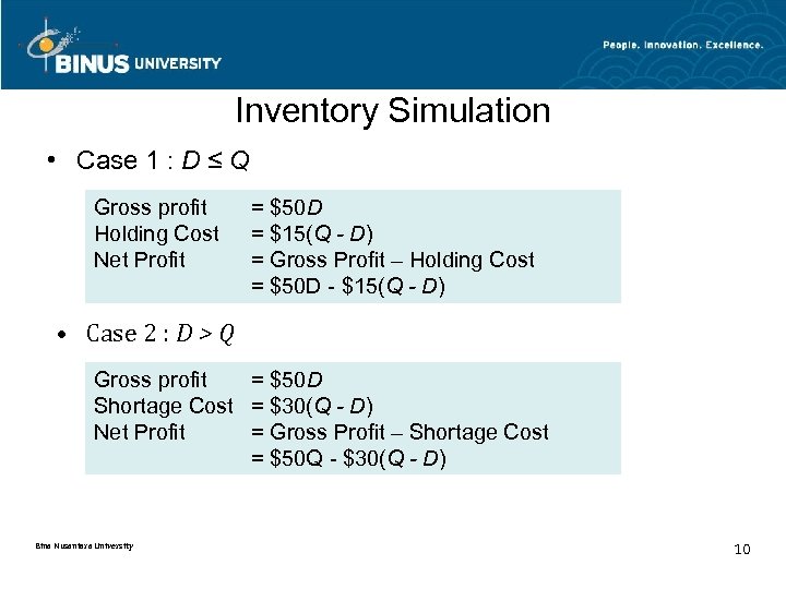Inventory Simulation • Case 1 : D ≤ Q Gross profit Holding Cost Net Profit = $50 D = $15(Q - D) = Gross Profit – Holding Cost = $50 D - $15(Q - D) • Case 2 : D > Q Gross profit = $50 D Shortage Cost = $30(Q - D) Net Profit = Gross Profit – Shortage Cost = $50 Q - $30(Q - D) Bina Nusantara University 10

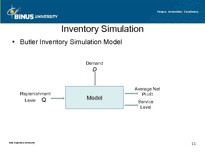Inventory Simulation • Butler Inventory Simulation Model Demand D Replenishment Level Q Bina Nusantara University Model Average Net Profit Service Level 11

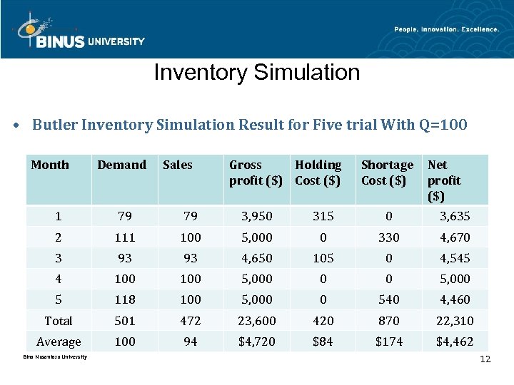Inventory Simulation • Butler Inventory Simulation Result for Five trial With Q=100 Month Demand Sales Gross Holding profit ($) Cost ($) Shortage Cost ($) Net profit ($) 1 79 79 3, 950 315 0 3, 635 2 111 100 5, 000 0 330 4, 670 3 93 93 4, 650 105 0 4, 545 4 100 5, 000 0 0 5, 000 5 118 100 5, 000 0 540 4, 460 Total 501 472 23, 600 420 870 22, 310 Average 100 94 $4, 720 $84 $174 $4, 462 Bina Nusantara University 12

Waiting Line Simulation • Example : Hammondsport Savings Bank ATM Waiting Line Hammondsport Savings Bank will open several new branch bank during the coming year. Each new branch is designed to have one automated teller machine (ATM). A concern is that during busy periods several customer may have to wait to use the ATM. This Concern prompted the bank to undertake a study of the waiting line system. The bank’s vise president want to determine whether one ATM will be sufficient. The bank established service guidelines for its ATM system stating that the average customer waiting time for an ATM should be one minute or less Bina Nusantara University 13

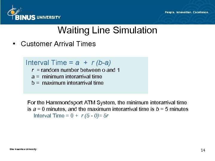Waiting Line Simulation • Customer Arrival Times Interval Time = a + r (b-a) r = random number between o and 1 a = minimum interarrival time b = maximum interarrival time For the Hammondsport ATM System, the minimum interarrival time is a = 0 minutes, and the maximum interarrival time is b = 5 minutes Interval Time = 0 + r (5 - 0)= 5 r Bina Nusantara University 14

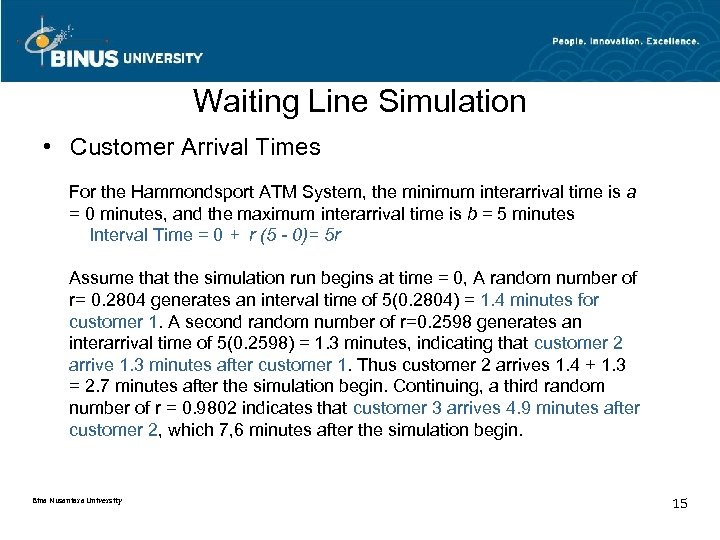Waiting Line Simulation • Customer Arrival Times For the Hammondsport ATM System, the minimum interarrival time is a = 0 minutes, and the maximum interarrival time is b = 5 minutes Interval Time = 0 + r (5 - 0)= 5 r Assume that the simulation run begins at time = 0, A random number of r= 0. 2804 generates an interval time of 5(0. 2804) = 1. 4 minutes for customer 1. A second random number of r=0. 2598 generates an interarrival time of 5(0. 2598) = 1. 3 minutes, indicating that customer 2 arrive 1. 3 minutes after customer 1. Thus customer 2 arrives 1. 4 + 1. 3 = 2. 7 minutes after the simulation begin. Continuing, a third random number of r = 0. 9802 indicates that customer 3 arrives 4. 9 minutes after customer 2, which 7, 6 minutes after the simulation begin. Bina Nusantara University 15

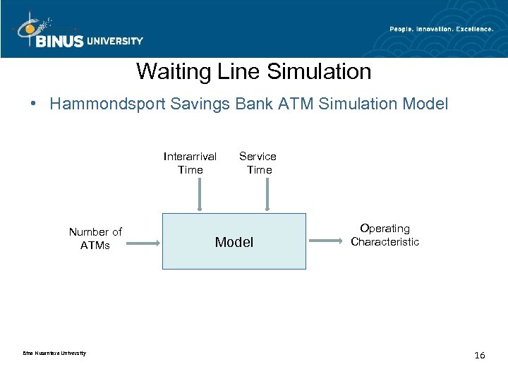Waiting Line Simulation • Hammondsport Savings Bank ATM Simulation Model Interarrival Time Number of ATMs Bina Nusantara University Service Time Model Operating Characteristic 16

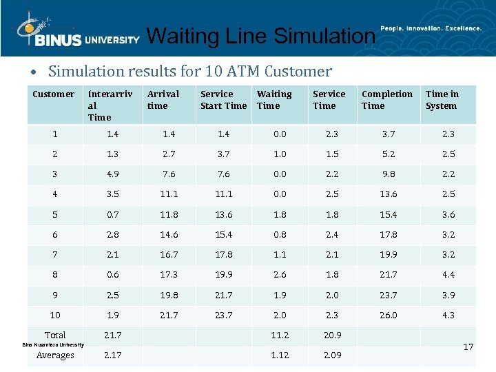Waiting Line Simulation • Simulation results for 10 ATM Customer Interarriv al Time Arrival time Service Waiting Start Time Service Time 1 1. 4 0. 0 2. 3 3. 7 2. 3 2 1. 3 2. 7 3. 7 1. 0 1. 5 5. 2 2. 5 3 4. 9 7. 6 0. 0 2. 2 9. 8 2. 2 4 3. 5 11. 1 0. 0 2. 5 13. 6 2. 5 5 0. 7 11. 8 13. 6 1. 8 15. 4 3. 6 6 2. 8 14. 6 15. 4 0. 8 2. 4 17. 8 3. 2 7 2. 1 16. 7 17. 8 1. 1 2. 1 19. 9 3. 2 8 0. 6 17. 3 19. 9 2. 6 1. 8 21. 7 4. 4 9 2. 5 19. 8 21. 7 1. 9 2. 0 23. 7 3. 9 10 1. 9 21. 7 23. 7 2. 0 2. 3 26. 0 4. 3 Total 21. 7 11. 2 20. 9 2. 17 1. 12 2. 09 Bina Nusantara University Averages Completion Time in System 17