Markets When Firms are Price Takers Jump to

Markets When Firms are Price Takers Jump to first page Copyright 2003 South-Western Thomson Learning. All rights reserved.

Conditions for a Market of Price Takers • • All firms produce an identical product. A large number of firms are in the market. Each firm supplies only a small portion of the total supplied to the market. No barriers to entry or exit exist. Jump to first page Copyright 2003 South-Western Thomson Learning. All rights reserved.

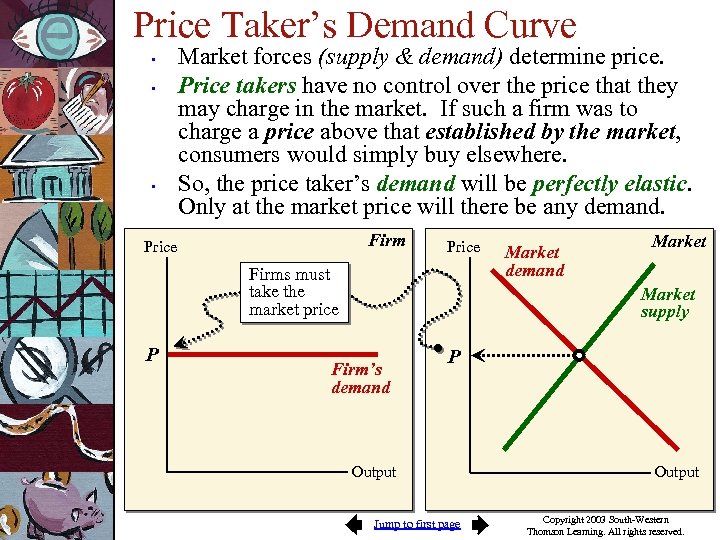Price Taker’s Demand Curve • • • Market forces (supply & demand) determine price. Price takers have no control over the price that they may charge in the market. If such a firm was to charge a price above that established by the market, consumers would simply buy elsewhere. So, the price taker’s demand will be perfectly elastic. Only at the market price will there be any demand. Firm Price Firms must take the market price P Market demand Market supply Firm’s demand P Output Jump to first page Output Copyright 2003 South-Western Thomson Learning. All rights reserved.

Output in the Short Run Jump to first page Copyright 2003 South-Western Thomson Learning. All rights reserved.

Marginal Revenue • Marginal Revenue is the change in total revenue divided by the change in output. Marginal (MR) Revenue • = change in total revenue change in output In a price taker market, marginal revenue (MR) = market price, because all units are sold at the same price (market price). Jump to first page Copyright 2003 South-Western Thomson Learning. All rights reserved.

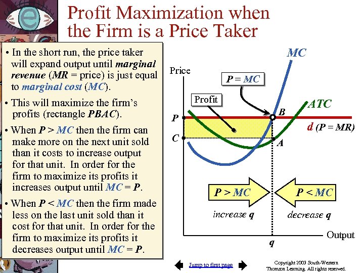Profit Maximization when the Firm is a Price Taker • In the short run, the price taker will expand output until marginal revenue (MR = price) is just equal to marginal cost (MC). • This will maximize the firm’s profits (rectangle PBAC). • When P > MC then the firm can make more on the next unit sold than it costs to increase output for that unit. In order for the firm to maximize its profits it increases output until MC = P. • When P < MC then the firm made less on the last unit sold than it cost for that unit. In order for the firm to maximize its profits it decreases output until MC = P. MC Price P = MC Profit B P ATC d (P = MR) C A P > MC P < MC increase q decrease q q Jump to first page Output Copyright 2003 South-Western Thomson Learning. All rights reserved.

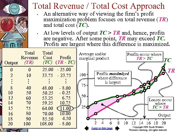Total Revenue / Total Cost Approach • • An alternative way of viewing the firm’s profit maximization problem focuses on total revenue (TR) and total cost (TC). At low levels of output TC > TR and, hence, profits are negative. After some point, TR may exceed TC. Profits are largest where this difference is maximized. Total Average and/or Profits occur where Profit Revenue Cost marginal product TR > TC TC (TC) (TR - TC) Output (TR) 25. 00 - 25. 00 0 0 TR Profits maximized 100 33. 75 - 23. 75 10 2 where difference. . . is largest 75 40 48. 00 - 8. 00 8 10 50 50. 25 - 0. 25 50 6. 75 12 53. 25 60 Losses occur 70 14 59. 25 10. 75 where 25 TC > TR 15 75 64. 00 11. 00 80 70. 00 16 Output 4. 50 90 18 85. 50 2 4 6 8 10 12 14 16 18 20 20 108. 00 - 8. 00 Jump to first page Copyright 2003 South-Western Thomson Learning. All rights reserved.

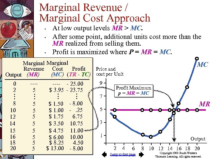Marginal Revenue / Marginal Cost Approach • • • At low output levels MR > MC. After some point, additional units cost more than the MR realized from selling them. Profit is maximized where P = MR = MC. Marginal Profit Price and Revenue Cost (MC) (TR - TC) cost per Unit Output (MR) 0 2. . . 8 10 12 14 15 16 18 20 ---5. . . 5 5 5 5 ---$ 3. 95. . . $ 1. 50 $ 1. 00 $ 1. 75 $ 3. 50 $ 4. 75 $ 6. 00 $ 8. 25 $ 13. 00 - 25. 00 - 23. 75. . . - 8. 00 -. 25 6. 75 10. 75 11. 00 10. 00 4. 50 - 8. 00 9 7 MC Profit Maximum p = MR = MC MR 5 3 1 Output 2 4 6 Jump to first page 8 10 12 14 16 18 20 Copyright 2003 South-Western Thomson Learning. All rights reserved.

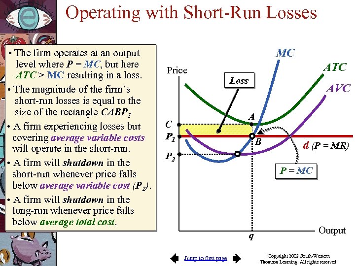Operating with Short-Run Losses • The firm operates at an output level where P = MC, but here ATC > MC resulting in a loss. • The magnitude of the firm’s short-run losses is equal to the size of the rectangle CABP 1 • A firm experiencing losses but covering average variable costs will operate in the short-run. • A firm will shutdown in the short-run whenever price falls below average variable cost (P 2). • A firm will shutdown in the long-run whenever price falls below average total cost. MC Price ATC Loss AVC A C P 1 B P 2 d (P = MR) P = MC q Jump to first page Output Copyright 2003 South-Western Thomson Learning. All rights reserved.

Output Adjustments in the Long Run Jump to first page Copyright 2003 South-Western Thomson Learning. All rights reserved.

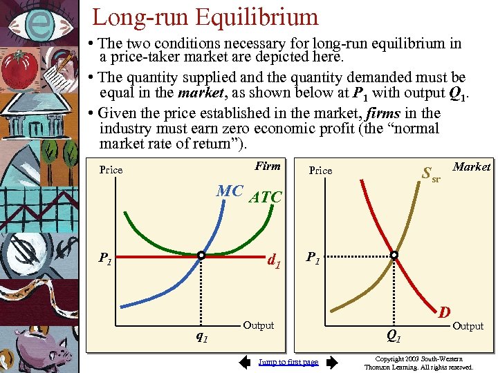Long-run Equilibrium • The two conditions necessary for long-run equilibrium in a price-taker market are depicted here. • The quantity supplied and the quantity demanded must be equal in the market, as shown below at P 1 with output Q 1. • Given the price established in the market, firms in the industry must earn zero economic profit (the “normal market rate of return”). Firm Price Ssr Price MC ATC P 1 d 1 q 1 Market P 1 Output Jump to first page D Q 1 Output Copyright 2003 South-Western Thomson Learning. All rights reserved.

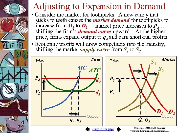Adjusting to Expansion in Demand • Consider the market for toothpicks. A new candy that sticks to teeth causes the market demand for toothpicks to increase from D 1 to D 2 … market price increases to P 2 … shifting the firm’s demand curve upward. At the higher price, firms expand output to q 2 and earn short-run profits. • Economic profits will draw competitors into the industry, shifting the market supply curve from S 1 to S 2. Firm Price S 1 Price MC ATC P 2 d 1 S 2 P 1 Market P 1 q 2 Output Jump to first page D 1 D 2 Q 1 Q 2 Output Copyright 2003 South-Western Thomson Learning. All rights reserved.

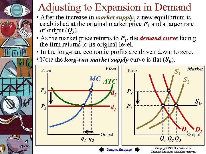Adjusting to Expansion in Demand • After the increase in market supply, a new equilibrium is established at the original market price P 1 and a larger rate of output (Q 3). • As the market price returns to P 1, the demand curve facing the firm returns to its original level. • In the long-run, economic profits are driven down to zero. • Note the long-run market supply curve is flat (Slr). Firm Price MC ATC P 2 d 2 q 1 q 2 P 1 Market S 2 P 2 d 1 P 1 S 1 Output Jump to first page Slr D 1 D 2 Q 1 Q 2 Q 3 Output Copyright 2003 South-Western Thomson Learning. All rights reserved.

The Case of Monopoly Jump to first page Copyright 2003 South-Western Thomson Learning. All rights reserved.

Monopoly • Monopoly is a market with: • • • high entry barriers, and, a single seller of a well-defined product for which there are no good substitutes. Only a few markets exist with a single seller but it is worth studying. • understanding monopoly theory also helps us understand markets with only a few sellers. Jump to first page Copyright 2003 South-Western Thomson Learning. All rights reserved.

Price and Output Under Monopoly • • As there is only one producer of a good or service in a market with a monopolist, the market demand curve is the monopolist’s demand curve. In order to maximize its profits, a monopolist will expand its output until marginal revenue just equals marginal cost. • The monopolist will charge the price along the demand curve consistent with that level of output. Jump to first page Copyright 2003 South-Western Thomson Learning. All rights reserved.

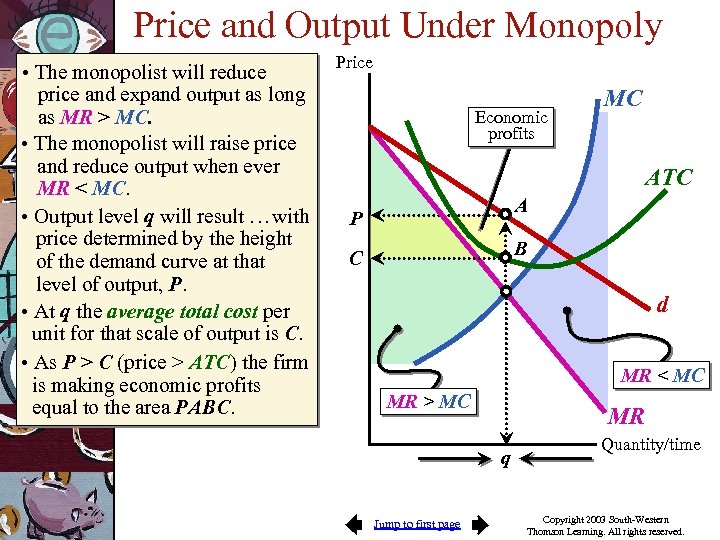Price and Output Under Monopoly • The monopolist will reduce price and expand output as long as MR > MC. • The monopolist will raise price and reduce output when ever MR < MC. • Output level q will result … with price determined by the height of the demand curve at that level of output, P. • At q the average total cost per unit for that scale of output is C. • As P > C (price > ATC) the firm is making economic profits equal to the area PABC. Price Economic profits MC ATC A P B C d MR < MC MR > MC MR q Jump to first page Quantity/time Copyright 2003 South-Western Thomson Learning. All rights reserved.

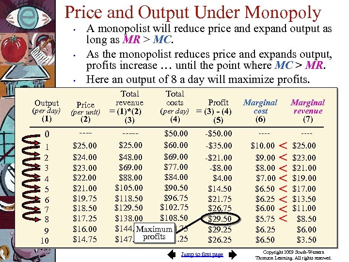Price and Output Under Monopoly • • • Output A monopolist will reduce price and expand output as long as MR > MC. As the monopolist reduces price and expands output, profits increase … until the point where MC > MR. Here an output of 8 a day will maximize profits. Price (per day) (per unit) 0 ---- 1 2 3 4 5 6 7 8 9 10 $25. 00 $24. 00 $23. 00 $22. 00 $21. 00 $19. 75 $18. 50 $17. 25 $16. 00 $14. 75 (1) (2) Total revenue = (1)*(2) (3) ----- Total costs Profit (per day) = (3) - (4) (5) $50. 00 $60. 00 $25. 00 $69. 00 $48. 00 $77. 00 $69. 00 $84. 00 $88. 00 $90. 50 $105. 00 $96. 75 $118. 50 $102. 75 $129. 50 $108. 50 $138. 00 $114. 75 $144. 00 Maximum $121. 25 $147. 50 profits -$50. 00 -$35. 00 -$21. 00 -$8. 00 $4. 00 $14. 50 $21. 75 $26. 75 $29. 50 $29. 25 $26. 25 Jump to first page Marginal cost (6) Marginal revenue (7) ---$10. 00 $9. 00 $8. 00 $7. 00 $6. 50 $6. 25 $6. 00 $5. 75 $6. 25 $6. 50 ---- < < < < $25. 00 $23. 00 $21. 00 $19. 00 $17. 00 $13. 50 $11. 00 $8. 50 $6. 00 $3. 50 Copyright 2003 South-Western Thomson Learning. All rights reserved.

Profits Under Monopoly • High entry barriers protect monopolists from competitive pressures. • • Monopolists can earn long-run profits. However even a monopolist will not always be able to earn profit. • When ATC is always above the demand curve, the monopolist will be unable to cover costs (unable to earn a profit). Jump to first page Copyright 2003 South-Western Thomson Learning. All rights reserved.

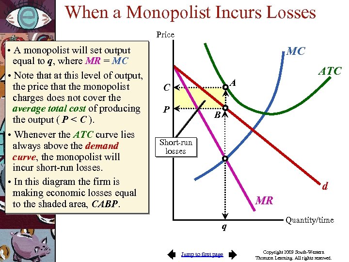When a Monopolist Incurs Losses Price • A monopolist will set output equal to q, where MR = MC • Note that at this level of output, the price that the monopolist charges does not cover the average total cost of producing the output ( P < C ). • Whenever the ATC curve lies always above the demand curve, the monopolist will incur short-run losses. • In this diagram the firm is making economic losses equal to the shaded area, CABP. MC ATC A C P B Short-run losses d MR q Jump to first page Quantity/time Copyright 2003 South-Western Thomson Learning. All rights reserved.

Characteristics of Oligopoly Jump to first page Copyright 2003 South-Western Thomson Learning. All rights reserved.

Characteristics of Oligopoly • A few characteristics of oligopoly: • • • small number of rival firms interdependence among firms substantial economies of scale significant barriers to entry products may be identical or differentiated Jump to first page Copyright 2003 South-Western Thomson Learning. All rights reserved.

Price and Output in the Case of Oligopoly Jump to first page Copyright 2003 South-Western Thomson Learning. All rights reserved.

Price and Output Under Oligopoly • No general theory exists for price and output under oligopoly. • • • If the firms operated independently, they would drive down the price to the per unit cost of production. If the firms colluded perfectly, the price would rise to the monopoly price. The outcome is usually between these two extremes. Jump to first page Copyright 2003 South-Western Thomson Learning. All rights reserved.

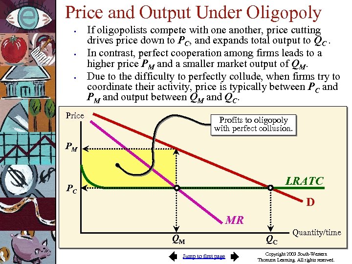Price and Output Under Oligopoly • • • If oligopolists compete with one another, price cutting drives price down to PC, and expands total output to QC. In contrast, perfect cooperation among firms leads to a higher price PM and a smaller market output of QM. Due to the difficulty to perfectly collude, when firms try to coordinate their activity, price is typically between PC and PM and output between QM and QC. Price Profits to oligopoly with perfect collusion. PM LRATC PC D MR QM Jump to first page QC Quantity/time Copyright 2003 South-Western Thomson Learning. All rights reserved.

Incentive to Collude • • • Oligopolists have a strong incentive to collude and raise their prices. However, each firm has an incentive to cheat by lowering price because the demand curve facing each firm is more elastic than the market demand curve. This conflict makes collusive agreements difficult to maintain. Jump to first page Copyright 2003 South-Western Thomson Learning. All rights reserved.

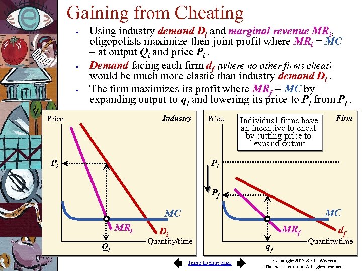Gaining from Cheating • • • Using industry demand Di and marginal revenue MRi, oligopolists maximize their joint profit where MRi = MC – at output Qi and price Pi. Demand facing each firm df (where no other firms cheat) would be much more elastic than industry demand Di. The firm maximizes its profit where MRf = MC by expanding output to qf and lowering its price to Pf from Pi. Industry Price Pi Price Individual firms have an incentive to cheat by cutting price to expand output Firm Pi Pf MC MC MRi Qi MRf Di Quantity/time Jump to first page qf df Quantity/time Copyright 2003 South-Western Thomson Learning. All rights reserved.

Obstacles to Collusion • • • As the number of firms in an oligopolistic market increases, the likelihood of effective collusion declines. When it is difficult to detect cheating (secret price cuts), effective collusion is less likely. Low entry barriers also make effective collusion less likely because profit attracts additional rivals. Unstable demand conditions lead to honest differences among firms about the size of shares and price that maximizes total profit. Rigorous enforcement of antitrust law makes collusion potentially more costly. Jump to first page Copyright 2003 South-Western Thomson Learning. All rights reserved.

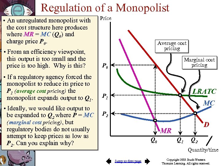Regulation of a Monopolist • An unregulated monopolist with the cost structure here produces where MR = MC (Q 0) and charge price P 0. Price Average cost pricing • From an efficiency viewpoint, this output is too small and the price is too high. Why is this? P 0 • If a regulatory agency forced the monopolist to reduce its price to P 1 (average cost pricing) the monopolist expands output to Q 1. P 1 • Ideally, we would like output to be expanded to Q 2 where P = MC (marginal cost pricing), but regulatory bodies do not usually attempt to keep prices as low as P 2. Can you explain why? Marginal cost pricing LRATC MC P 2 D MR Q 0 Q 1 Q 2 Quantity/time Jump to first page Copyright 2003 South-Western Thomson Learning. All rights reserved.

Problems with Government Intervention • Problems with price regulation: • • Lack of information – do regulators know the cost structures behind the firm’s real ATC? Cost shifting – with P = ATC, do monopolists have much incentive to keep costs low? Special interest influence – will monopolists have an incentive to influence the decisions of regulatory bodies? Problem with government production: • • • Less incentive to minimize costs and adopt new technologies. Fewer incentives to satisfy customers, improve quality, and introduce new products. Political considerations may influence decision making of firm. Jump to first page Copyright 2003 South-Western Thomson Learning. All rights reserved.

Monopolistic Competition Competitive Price-Searcher Markets Jump to first page Copyright 2003 South-Western Thomson Learning. All rights reserved.

Competitive Price-Searcher Markets • Firms in price-searcher markets with low entry barriers face a downward sloping demand curve. • • • Firms are free to set price, but face strong competitive pressure. Competition exists from existing firms and potential rivals An alternative term for such markets is monopolistic competition. Jump to first page Copyright 2003 South-Western Thomson Learning. All rights reserved.

Product Differentiation • Price-searchers produce differentiated products – products that differ in design, dependability, location, ease of purchase, etc. • Rival firms produce similar products (good substitutes) and therefore each firm confronts a highly elastic demand curve. Jump to first page Copyright 2003 South-Western Thomson Learning. All rights reserved.

Price and Output • A profit-maximizing price searcher will expand output as long as marginal revenue exceeds marginal cost. • • Price will be lowered and output expanded until MR = MC The price charged by a price searcher will be greater than its marginal cost. Jump to first page Copyright 2003 South-Western Thomson Learning. All rights reserved.

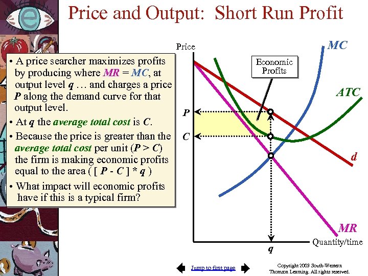Price and Output: Short Run Profit MC Price • A price searcher maximizes profits by producing where MR = MC, at output level q … and charges a price P along the demand curve for that output level. P • At q the average total cost is C. • Because the price is greater than the C average total cost per unit (P > C) the firm is making economic profits equal to the area ( [ P - C ] * q ) • What impact will economic profits have if this is a typical firm? Economic Profits ATC d MR q Jump to first page Quantity/time Copyright 2003 South-Western Thomson Learning. All rights reserved.

Profits and Losses in the Long Run • If firms are making economic profits, then rival firms will be attracted to the market. • • • Economic losses will cause price searchers to exit from the market. • • The entry of new firms will expand supply and lower price. The demand curve of each will shift inward until the economic profits are eliminated. Demand for the remaining firms’ output will rise until the losses have been eliminated, ending the incentive to exit. Competitive price searchers can make either profits or losses in the short run, but only zero economic profit in the long run. Jump to first page Copyright 2003 South-Western Thomson Learning. All rights reserved.

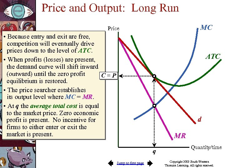Price and Output: Long Run MC Price • Because entry and exit are free, competition will eventually drive prices down to the level of ATC. • When profits (losses) are present, the demand curve will shift inward (outward) until the zero profit C=P equilibrium is restored. • The price searcher establishes its output level where MC = MR. • At q the average total cost is equal to the market price. Zero economic profit is present. No incentive for firms to either enter or exit the market is present. ATC d MR q Jump to first page Quantity/time Copyright 2003 South-Western Thomson Learning. All rights reserved.

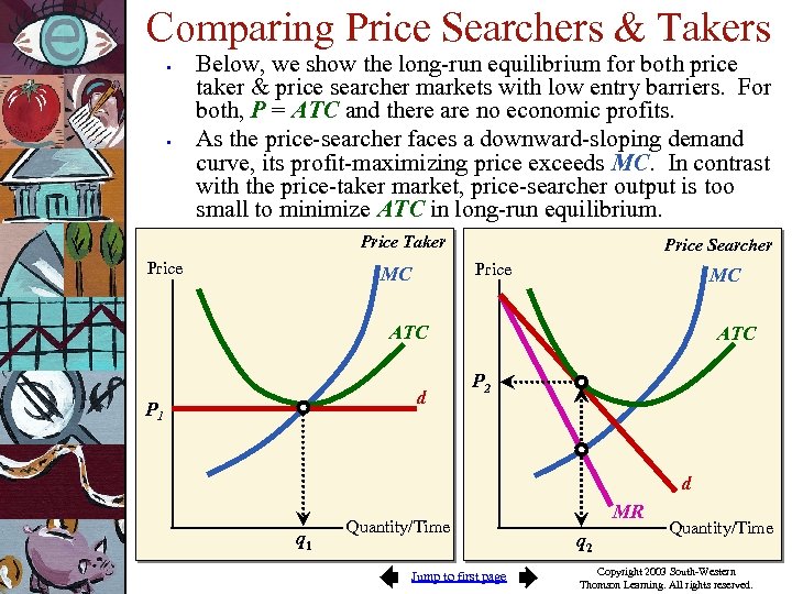Comparing Price Searchers & Takers • • Below, we show the long-run equilibrium for both price taker & price searcher markets with low entry barriers. For both, P = ATC and there are no economic profits. As the price-searcher faces a downward-sloping demand curve, its profit-maximizing price exceeds MC. In contrast with the price-taker market, price-searcher output is too small to minimize ATC in long-run equilibrium. Price Taker Price Searcher Price MC MC ATC d P 1 ATC P 2 d q 1 Quantity/Time Jump to first page MR q 2 Quantity/Time Copyright 2003 South-Western Thomson Learning. All rights reserved.

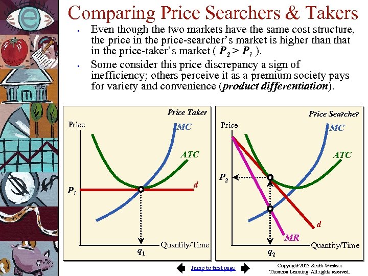Comparing Price Searchers & Takers • • Even though the two markets have the same cost structure, the price in the price-searcher’s market is higher than that in the price-taker’s market ( P 2 > P 1 ). Some consider this price discrepancy a sign of inefficiency; others perceive it as a premium society pays for variety and convenience (product differentiation). Price Taker Price Searcher Price MC MC ATC d P 1 ATC P 2 d q 1 Quantity/Time Jump to first page MR q 2 Quantity/Time Copyright 2003 South-Western Thomson Learning. All rights reserved.

Allocative Efficiency • • Allocative efficiency is achieved when the most desired goods are produced at the lowest possible cost. Criticism of traditional theory of competitive price-searcher markets: • • • price > marginal cost at the profit maximizing output level per-unit cost may not be minimized excessive advertising is encouraged Jump to first page Copyright 2003 South-Western Thomson Learning. All rights reserved.

Allocative Efficiency • Recently economists have been more positive about competitive price-searcher markets. • • • Consumers may value a wider variety of styles and quality (product differentiation). Advertising often reduces search time and provides valuable information. Price searchers have an incentive to innovate and operate efficiently. Jump to first page Copyright 2003 South-Western Thomson Learning. All rights reserved.

A Special Case: Price Discrimination Jump to first page Copyright 2003 South-Western Thomson Learning. All rights reserved.

Price Discrimination • Price discrimination: When a seller charges different consumers different prices for the same good or service. • Price discrimination can only occur when a price searcher is able to: • • identify groups of customers with different elasticities of demand prevent customers re-trading the product. Jump to first page Copyright 2003 South-Western Thomson Learning. All rights reserved.

Price Discrimination • Sellers may gain from price discrimination by charging: • • • higher prices to groups of customers with more inelastic demand lower prices to groups of customers with more elastic demand Price discrimination generally leads to more output and additional gains from trade. Jump to first page Copyright 2003 South-Western Thomson Learning. All rights reserved.

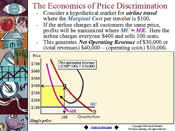The Economics of Price Discrimination • • • Consider a hypothetical market for airline travel where the Marginal Cost per traveler is $100. If the airline charges all customers the same price, profits will be maximized where MC = MR. Here the airline charges everyone $400 and sells 100 seats. This generates Net Operating Revenue of $30, 000 or (total revenues) $40, 000 – (operating costs) $10, 000. Price $700 Net operating revenue ($300*100) = $30, 000 $600 $500 $400 $300 $200 MC $100 Single price MR 100 D Quantity/time Jump to first page Copyright 2003 South-Western Thomson Learning. All rights reserved.

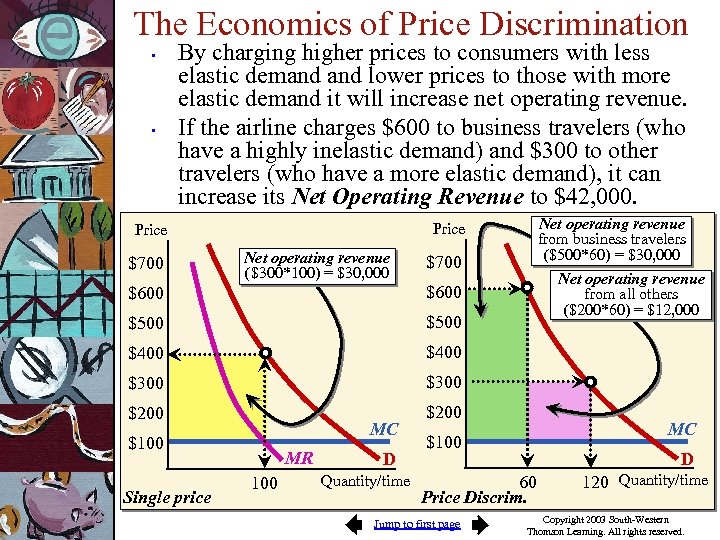The Economics of Price Discrimination • • By charging higher prices to consumers with less elastic demand lower prices to those with more elastic demand it will increase net operating revenue. If the airline charges $600 to business travelers (who have a highly inelastic demand) and $300 to other travelers (who have a more elastic demand), it can increase its Net Operating Revenue to $42, 000. $700 Net operating revenue from business travelers ($500*60) = $30, 000 Price Net operating revenue ($300*100) = $30, 000 $700 $600 $500 $400 $300 $200 Net operating revenue from all others ($200*60) = $12, 000 $200 MC $100 Single price MR 100 D Quantity/time MC $100 D 60 Price Discrim. Jump to first page 120 Quantity/time Copyright 2003 South-Western Thomson Learning. All rights reserved.

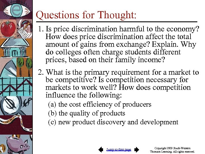Questions for Thought: 1. Is price discrimination harmful to the economy? How does price discrimination affect the total amount of gains from exchange? Explain. Why do colleges often charge students different prices, based on their family income? 2. What is the primary requirement for a market to be competitive? Is competition necessary for markets to work well? How does competition influence the following: (a) the cost efficiency of producers (b) the quality of products (c) new product discovery and development Jump to first page Copyright 2003 South-Western Thomson Learning. All rights reserved.

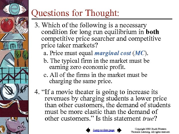Questions for Thought: 3. Which of the following is a necessary condition for long run equilibrium in both competitive price searcher and competitive price taker markets? a. Price must equal marginal cost (MC). b. The typical firm in the market must be earning zero economic profit. c. All of the firms in the market must be charging the same price. 4. “If a movie theater is going to increase its revenues by charging students a lower price than other customers, the demand of students must be more elastic than the demand of other customers. ” Is this statement true? Jump to first page Copyright 2003 South-Western Thomson Learning. All rights reserved.

Questions for Thought: 5. Which of the following indicates that a firm operating in the highly competitive retail sector is providing goods and services that consumers value highly relative to their cost? a. The firm is making losses and its sales are declining. b. The wages earned by the employees of the firm are low. c. The firm is highly profitable and its sales have grown rapidly. Jump to first page Copyright 2003 South-Western Thomson Learning. All rights reserved.