517fd21fe444b7e2be0e971aba4dfcf0.ppt
- Количество слайдов: 50

Markets Are a mechanism that brings buyers and sellers together to exchange goods, services, and resources. It is a device for allocating or rationing goods, services, and resources. • A competitive market: – Many buyers and sellers; Same good or service • Product market: where consumer goods are bought and sold. Business firms are the seller, consumers are the buyers • Resource market: where the resource services are bought and sold. Resource owners(consumers) are the sellers and business firms are the buyers • Five key elements: – – Demand curve, Supply curve Demand supply curve shifts Market equilibrium Changes in the market equilibrium
Definition: relationship between the price and the quantity demanded of a good. • Quantity demanded: amount of an item that buyers are willing and able to purchase over a certain time period, at a specific price, ceteris paribus.
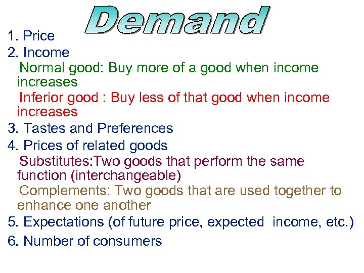
1. Price 2. Income Normal good: Buy more of a good when income increases Inferior good : Buy less of that good when income increases 3. Tastes and Preferences 4. Prices of related goods Substitutes: Two goods that perform the same function (interchangeable) Complements: Two goods that are used together to enhance one another 5. Expectations (of future price, expected income, etc. ) 6. Number of consumers
1. Price The variables below this line will be held constant (ceteris Paribus) 2. Income Normal good: Wish to buy more of a good when income increases Inferior good : Wish to buy less of that good when income increases 3. Tastes and Preferences 4. Prices of related goods Substitutes: Two goods that perform the same function (interchangeable) Complements: Two goods that are used together to enhance one another 5. Expectations (of future price, expected income, etc. ) 6. Number of consumers
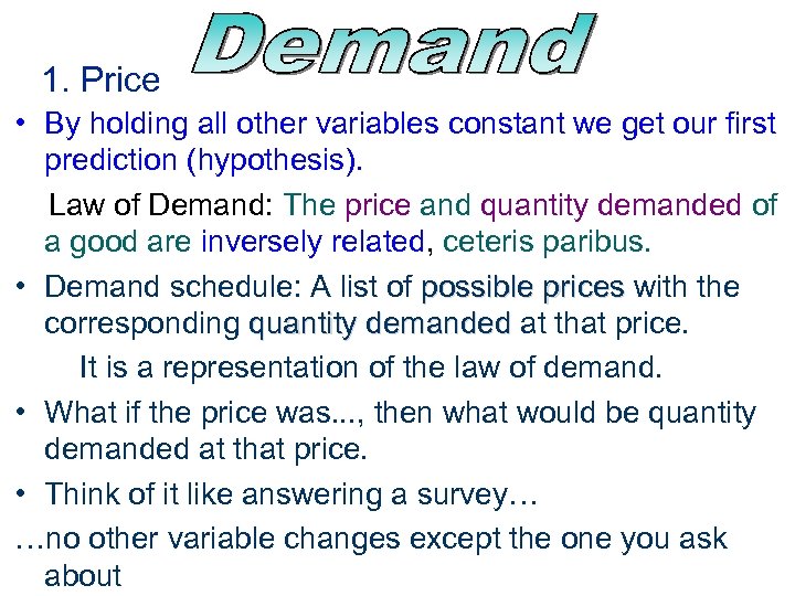
1. Price • By holding all other variables constant we get our first prediction (hypothesis). Law of Demand: The price and quantity demanded of a good are inversely related, ceteris paribus. • Demand schedule: A list of possible prices with the corresponding quantity demanded at that price. It is a representation of the law of demand. • What if the price was. . . , then what would be quantity demanded at that price. • Think of it like answering a survey… …no other variable changes except the one you ask about
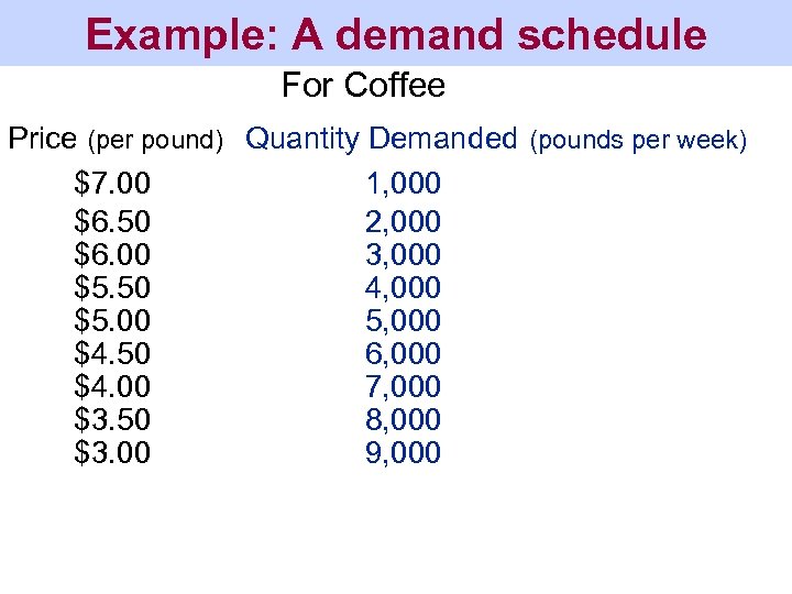
Example: A demand schedule For Coffee Price (per pound) Quantity Demanded (pounds per week) $7. 00 1, 000 $6. 50 2, 000 $6. 00 3, 000 $5. 50 4, 000 $5. 00 5, 000 $4. 50 6, 000 $4. 00 7, 000 $3. 50 8, 000 $3. 00 9, 000
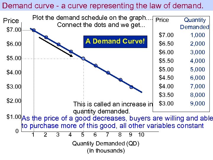
Demand curve - a curve representing the law of demand. Plot the demand schedule on the graph. . Price Connect the dots and we get. . . Price $7. 00 A Demand Curve! $6. 50 $6. 00 $5. 50 $5. 00 $4. 50 $4. 00 $3. 50 This is called an increase in $3. 00 $6. 00 $5. 00 $4. 00 $3. 00 $2. 00 quantity demanded. $1. 00 As 0 Quantity Demanded 1, 000 2, 000 3, 000 4, 000 5, 000 6, 000 7, 000 8, 000 9, 000 the price of a good decreases, buyers are willing and able decreases to purchase more of this good, all other variables constant 1 2 3 4 5 6 7 8 9 10 Quantity Demanded (QD) (In thousands)
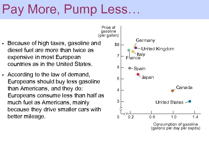
Pay More, Pump Less… Price of gasoline (per gallon) § § Because of high taxes, gasoline and diesel fuel are more than twice as expensive in most European countries as in the United States. According to the law of demand, Europeans should buy less gasoline than Americans, and they do: Europeans consume less than half as much fuel as Americans, mainly because they drive smaller cars with better mileage. $8 7 6 Germany United Kingdom Italy France Spain Japan 5 Canada 4 3 0 United States 0. 2 0. 6 1. 0 1. 4 Consumption of gasoline (gallons per day per capita)
What about the other variables? • To construct a single demand curve a number of variables are held constant. . . (Income, Expectations, prices of related goods, etc) • What would happen to the demand curve if one of these variables were to change? • Example: Suppose consumers income increases and coffee is a normal good. People will want to buy more coffee. . . not just at one specific price but at all prices!
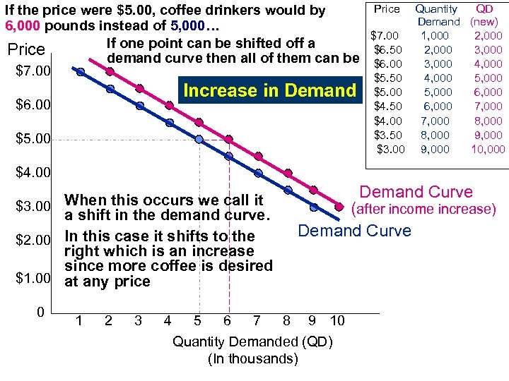
If the price were $5. 00, coffee drinkers would by 6, 000 pounds instead of 5, 000… If one point can be shifted off a Price demand curve then all of them can be $7. 00 Increase in Demand $6. 00 $5. 00 Price Quantity QD Demand (new) $7. 00 1, 000 2, 000 $6. 50 2, 000 3, 000 $6. 00 3, 000 4, 000 $5. 50 4, 000 5, 000 $5. 00 5, 000 6, 000 $4. 50 6, 000 7, 000 $4. 00 7, 000 8, 000 $3. 50 8, 000 9, 000 $3. 00 9, 000 10, 000 $4. 00 $3. 00 When this occurs we call it a shift in the demand curve. $2. 00 In this case it shifts to the right which is an increase since more coffee is desired $1. 00 at any price 0 1 2 3 4 Demand Curve (after income increase) Demand Curve 5 6 7 8 9 10 Quantity Demanded (QD) (In thousands)
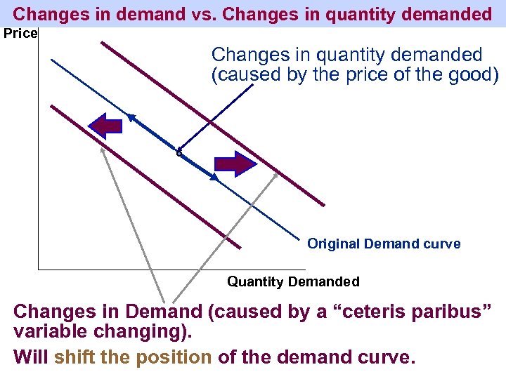
Changes in demand vs. Changes in quantity demanded Price Changes in quantity demanded (caused by the price of the good) Original Demand curve Quantity Demanded Changes in Demand (caused by a “ceteris paribus” variable changing). Will shift the position of the demand curve.
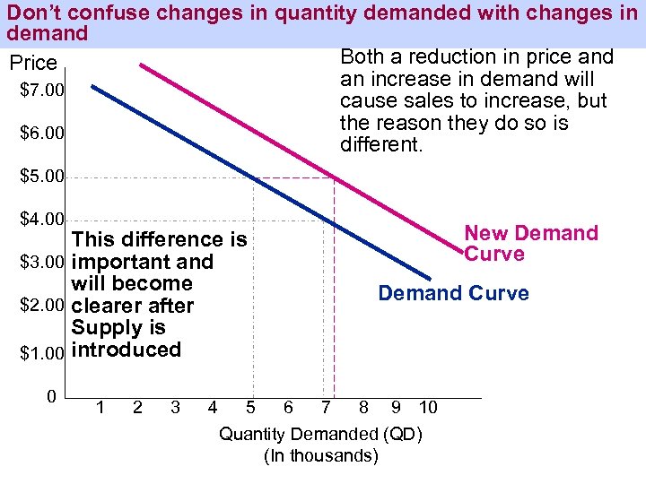
Don’t confuse changes in quantity demanded with changes in demand Both a reduction in price and Price an increase in demand will $7. 00 cause sales to increase, but the reason they do so is $6. 00 different. $5. 00 $4. 00 This difference is $3. 00 important and will become $2. 00 clearer after Supply is $1. 00 introduced 0 1 2 3 4 New Demand Curve 5 6 7 8 9 10 Quantity Demanded (QD) (In thousands)
How do the other “ceteris paribus” variables affect the demand curve? 1. Prices of related goods Substitutes • If the price of tea increases, then consumers will wish increases to buy more coffee. . . since coffee is now relatively cheaper compared to tea. In general, as the price of a substitute good increases, the demand for the other good increases • Therefore, there is a direct relationship between the demand for a good and the price of a substitute good. • Other examples: Foreign cars - American cars, chicken - beef, Coke - Pepsi, etc. • Consumers always purchase more of the good that is now cheaper relative to the other good.
“Ceteris paribus” Variables 1. Prices of related goods Complements • If the price of sugar and cream were to increase, then increase consumers will desire to buy less coffee because the two joined products (Coffee-(sugar-cream)) now are more expensive. As the price of a complementary good increases, the increases demand for the other good decreases • Therefore, there is an inverse relationship between the demand for a good and the price of a complementary good. • Other examples: Cars - gasoline, Computers software, Compact discs - Compact disc players, hot dogs - mustard
“Ceteris paribus” Variables 2. Tastes & Preferences If consumers prefer a good there is an increase in demand. If a good falls out of favor there is a decrease in demand Advertising could have an effect on tastes & preferences 3. Expectations Of future prices, availability of goods, income. If you believe that prices will increase in the future, you will want to buy more today before the price increase (increase in demand) Important for prices of commodities, stocks, and bonds 4. # of consumers: more consumers, increase in demand
• Definition: relationship between the price of a good and the quantity supplied of a good. • Quantity supplied: amount of an item that sellers are willing and able to make available to market over a certain period, at a specific price, ceteris paribus.
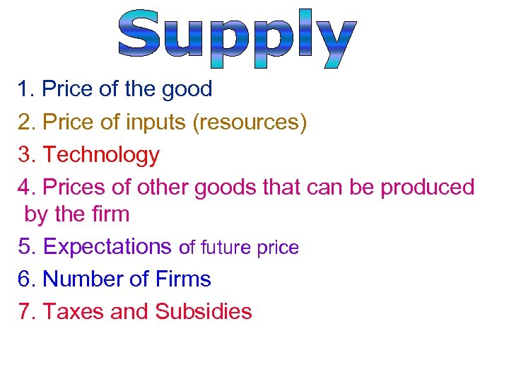
1. Price of the good 2. Price of inputs (resources) 3. Technology 4. Prices of other goods that can be produced by the firm 5. Expectations of future price 6. Number of Firms 7. Taxes and Subsidies
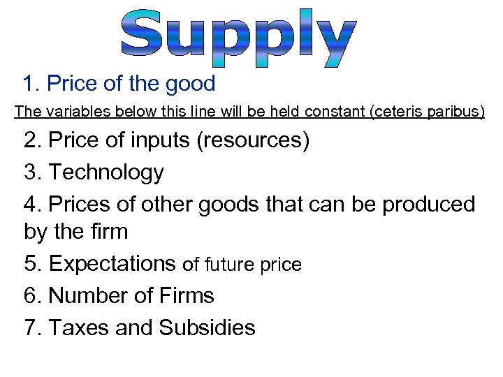
1. Price of the good The variables below this line will be held constant (ceteris paribus) 2. Price of inputs (resources) 3. Technology 4. Prices of other goods that can be produced by the firm 5. Expectations of future price 6. Number of Firms 7. Taxes and Subsidies
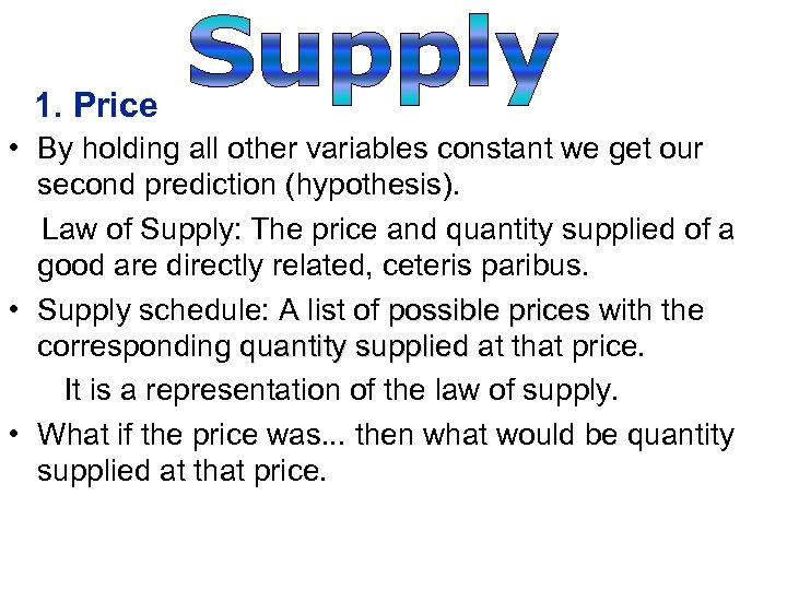
1. Price • By holding all other variables constant we get our second prediction (hypothesis). Law of Supply: The price and quantity supplied of a good are directly related, ceteris paribus. • Supply schedule: A list of possible prices with the corresponding quantity supplied at that price. It is a representation of the law of supply. • What if the price was. . . then what would be quantity supplied at that price.
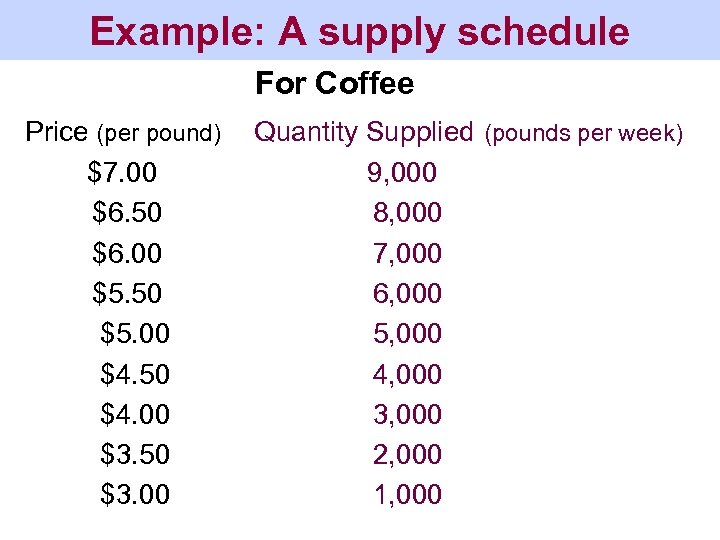
Example: A supply schedule For Coffee Price (per pound) $7. 00 $6. 50 $6. 00 $5. 50 $5. 00 $4. 50 $4. 00 $3. 50 $3. 00 Quantity Supplied (pounds per week) 9, 000 8, 000 7, 000 6, 000 5, 000 4, 000 3, 000 2, 000 1, 000
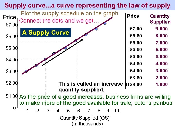
Supply curve. . . a curve representing the law of supply Plot the supply schedule on the graph. . . Price Connect the dots and we get… $7. 00 $6. 00 A Supply $5. 00 $4. 00 $3. 00 $2. 00 $7. 00 Curve $6. 50 $6. 00 $5. 50 $5. 00 $4. 50 $4. 00 $3. 50 This is called an increase in $3. 00 quantity supplied. $1. 00 As 0 Quantity Supplied 9, 000 8, 000 7, 000 6, 000 5, 000 4, 000 3, 000 2, 000 1, 000 the price of a good increases, business firms are willing increases to make more of the good available for sale, ceteris paribus sale 1 2 3 4 5 6 7 8 9 10 Quantity Supplied (QS) (In thousands)
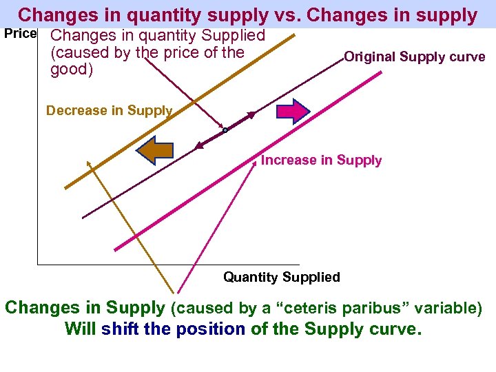
Changes in quantity supply vs. Changes in supply Price Changes in quantity Supplied (caused by the price of the good) Original Supply curve Decrease in Supply Increase in Supply Quantity Supplied Changes in Supply (caused by a “ceteris paribus” variable) Will shift the position of the Supply curve.
How do the “ceteris paribus” variables affect the Supply curve? • Price of inputs (resources) If the price of an input increases (labor, materials, etc) this makes a good more expensive to produce (raises costs). This lowers the potential profit of the firm so they will wish to decrease the supply of the good • Opposite example: The decline in the price of computer processors and chips makes costs decline for computer manufacturers and they increase supply • Summary: A decline in input prices increases supply. A rise in input prices decreases supply.
“Ceteris paribus” variables (Supply) • Technology. . . allows a firm to produce the same amount of a good with less resources, which results in lower costs and an increase in supply • Price of other goods the firm can produce. . . Example: If a farmer who grows coffee beans finds that another crop will pay them more… … they devote less land to coffee(a decrease in supply of coffee) and more land to the other crop • Expectations. . . of future prices If firms expect higher prices in the future they will make less available today (decrease in supply). Why? So they will have more to sell in the future (at the higher prices
“Ceteris paribus” variables (supply) • Number of firms The more firms that produce the good the greater is the supply of the good (more it shifts to the right) • Taxes and Subsidies Excise taxes. . . a tax on a good (gas, cigarette, etc) • An increase in excise taxes will raise the cost of the good, lower potential profits, cause a decrease in supply • A subsidy gives money (directly or indirectly) to firms, lowers the cost of the good and will increase supply. • Examples: Public colleges and universities receive money from state governments. • Immunizations are also subsidized by the government
Market Equilibrium • Equilibrium: Definition At rest, no tendency to change, forces in balance. • Market equilibrium. − the price, once reached, when there will be no tendency to change. − Also the price the market comes to rest at and where there are forces in balance. • This can only occur when Quantity demand (QD) = Quantity supplied (QS) • Price is a rationing device… …based on willingness and ability to pay
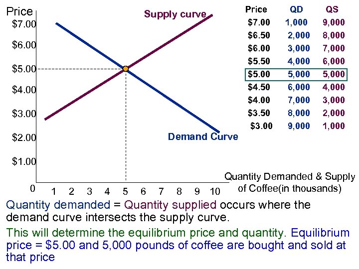
Price Supply curve $7. 00 $6. 00 $5. 00 $4. 00 $3. 00 Price $7. 00 $6. 50 $6. 00 $5. 50 $5. 00 $4. 50 $4. 00 $3. 50 $3. 00 QD 1, 000 2, 000 3, 000 4, 000 5, 000 6, 000 7, 000 8, 000 9, 000 QS 9, 000 8, 000 7, 000 6, 000 5, 000 4, 000 3, 000 2, 000 1, 000 Demand Curve $2. 00 $1. 00 0 1 2 3 4 5 6 7 8 Quantity Demanded & Supply of Coffee(in thousands) 9 10 Quantity demanded = Quantity supplied occurs where the demand curve intersects the supply curve. This will determine the equilibrium price and quantity. Equilibrium price = $5. 00 and 5, 000 pounds of coffee are bought and sold at that price
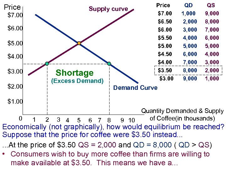
Price Supply curve $7. 00 $6. 00 $5. 00 $4. 00 $3. 00 Shortage (Excess Demand) $2. 00 Price $7. 00 $6. 50 $6. 00 $5. 50 $5. 00 $4. 50 $4. 00 $3. 50 $3. 00 QD 1, 000 2, 000 3, 000 4, 000 5, 000 6, 000 7, 000 8, 000 9, 000 QS 9, 000 8, 000 7, 000 6, 000 5, 000 4, 000 3, 000 2, 000 1, 000 Demand Curve $1. 00 0 1 2 3 4 5 6 7 8 Quantity Demanded & Supply of Coffee(in thousands) 9 10 Economically (not graphically), how would equilibrium be reached? Suppose that the price for coffee were $3. 50 instead. . . At the price of $3. 50 QS = 2, 000 and QD = 8, 000 ( QD > QS) • Consumers wish to buy more coffee than firms are willing to make available at $3. 50. This means we have a. . .
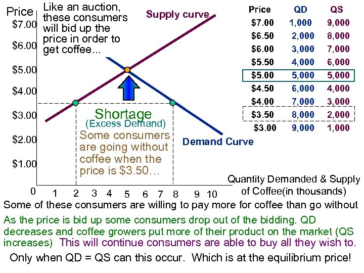
Price Like an auction, these consumers $7. 00 will bid up the Supply curve price in order to $6. 00 get coffee. . . $5. 00 $4. 00 Shortage $3. 00 (Excess Demand) Some consumers are going without coffee when the price is $3. 50… $2. 00 $1. 00 0 1 2 3 4 5 6 7 8 Price $7. 00 $6. 50 $6. 00 $5. 50 $5. 00 $4. 50 $4. 00 $3. 50 $3. 00 QD 1, 000 2, 000 3, 000 4, 000 5, 000 6, 000 7, 000 8, 000 9, 000 QS 9, 000 8, 000 7, 000 6, 000 5, 000 4, 000 3, 000 2, 000 1, 000 Demand Curve Quantity Demanded & Supply of Coffee(in thousands) 9 10 Some of these consumers are willing to pay more for coffee than go without As the price is bid up some consumers drop out of the bidding. QD decreases and coffee growers put more of their product on the market (QS increases) This will continue consumers are able to buy all they wish to. Only when QD = QS can this occur. Which is at the equilibrium price!
Economics in Action The Price of Admission: • Compare the box office price for a recent Justin Timberlake concert in Miami, Florida, to the Stub. Hub. com price for seats in the same location: $88. 50 versus $155. • Why is there such a big difference in prices? For major events, buying tickets from the box office means waiting in very long lines. Ticket buyers who use Internet resellers have decided that the opportunity cost of their time is too high to spend waiting in line. For those major events with online box offices selling tickets at face value, tickets often sell out within minutes. • In this case, some people who want to go to the concert badly but have missed out on the opportunity to buy cheaper tickets from the online box office are willing to pay the higher Internet reseller price.
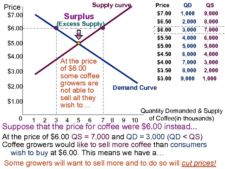
Supply curve Price $7. 00 Surplus (Excess Supply) $6. 00 $5. 00 $4. 00 At the price of $6. 00 some coffee growers are not able to sell all they wish to… $3. 00 $2. 00 $1. 00 0 1 2 3 4 5 6 Price $7. 00 $6. 50 $6. 00 $5. 50 $5. 00 $4. 50 $4. 00 $3. 50 $3. 00 QD 1, 000 2, 000 3, 000 4, 000 5, 000 6, 000 7, 000 8, 000 9, 000 QS 9, 000 8, 000 7, 000 6, 000 5, 000 4, 000 3, 000 2, 000 1, 000 Demand Curve 7 8 Quantity Demanded & Supply of Coffee(in thousands) 9 10 Suppose that the price for coffee were $6. 00 instead. . . At the price of $6. 00 QS = 7, 000 and QD = 3, 000 (QD < QS) Coffee growers would like to sell more coffee than consumers wish to buy at $6. 00. This means we have a… Some growers will want to sell more and to do so will cut prices!
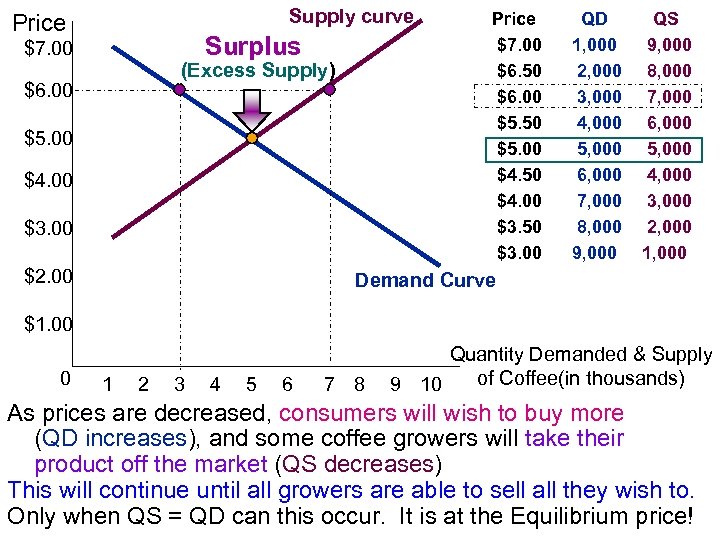
Supply curve Price Surplus $7. 00 (Excess Supply) $6. 00 $5. 00 $4. 00 $3. 00 $2. 00 Price $7. 00 $6. 50 $6. 00 $5. 50 $5. 00 $4. 50 $4. 00 $3. 50 $3. 00 QD 1, 000 2, 000 3, 000 4, 000 5, 000 6, 000 7, 000 8, 000 9, 000 QS 9, 000 8, 000 7, 000 6, 000 5, 000 4, 000 3, 000 2, 000 1, 000 Demand Curve $1. 00 0 1 2 3 4 5 6 7 8 Quantity Demanded & Supply of Coffee(in thousands) 9 10 As prices are decreased, consumers will wish to buy more (QD increases), and some coffee growers will take their product off the market (QS decreases) This will continue until all growers are able to sell all they wish to. Only when QS = QD can this occur. It is at the Equilibrium price!

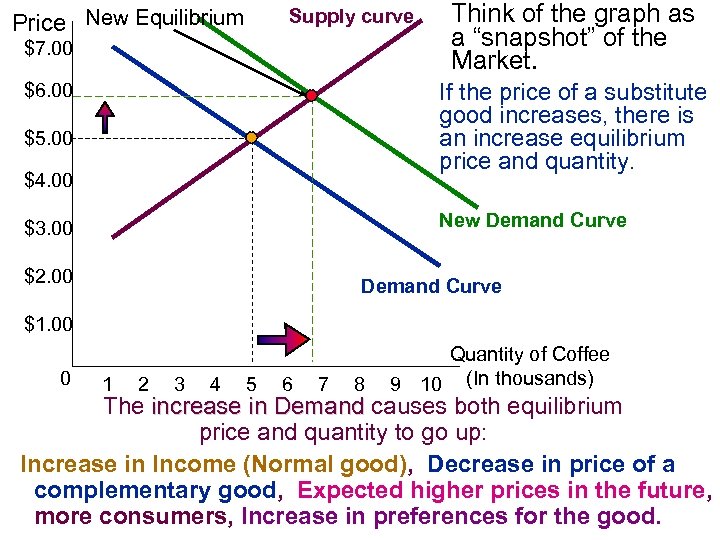
Supply curve Price New Equilibrium $7. 00 Think of the graph as a “snapshot” of the Market. If the price of a substitute good increases, there is an increase equilibrium price and quantity. $6. 00 $5. 00 $4. 00 New Demand Curve $3. 00 $2. 00 Demand Curve $1. 00 0 1 2 3 4 5 6 7 8 Quantity of Coffee 9 10 (In thousands) The increase in Demand causes both equilibrium If something changes(the quantity or go up: price and Supply to Demand curve shifts) in the Market the “snapshot” good), Decrease in price of a Increase in Income (Normal will change. . . Example: If the good, Expected higher good) increases, complementary price of tea(a substitute prices in the future, more consumers, Increase coffee (increase in the good. consumers will want more in preferences for demand)
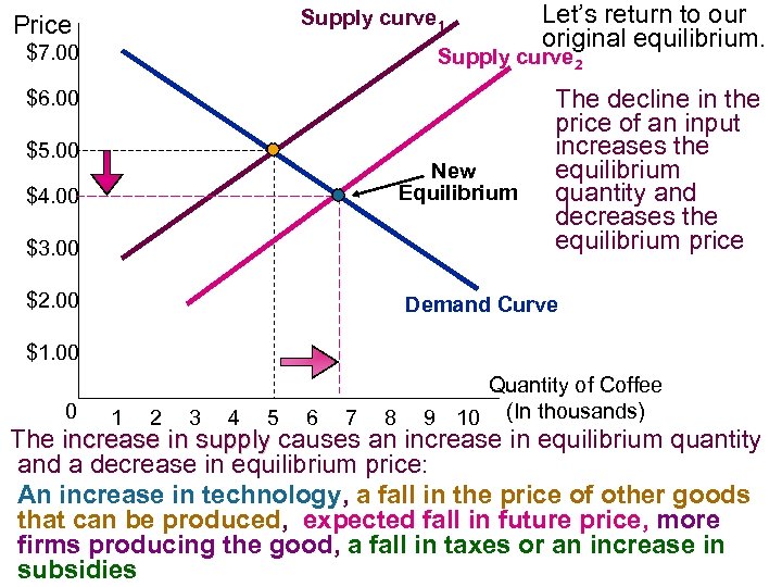
Supply curve 1 Price $7. 00 Let’s return to our original equilibrium. Supply curve 2 $6. 00 $5. 00 New Equilibrium $4. 00 $3. 00 $2. 00 The decline in the price of an input increases the equilibrium quantity and decreases the equilibrium price Demand Curve $1. 00 0 1 2 3 4 5 6 7 8 Quantity of Coffee 9 10 (In thousands) The increase in supply causes an increase in equilibrium quantity increase Suppose thein supply land(for growing coffee) decreases. . . price of and a decrease in equilibrium price: . . . the declinein technology, aan input will increase the An increase in the price of fall in the price of other goods profitability of coffee growers fall will want to produce that can be produced, expected whoin future price, more firms producing the good, a fall in taxes or an increase in more (increase in supply)… subsidies
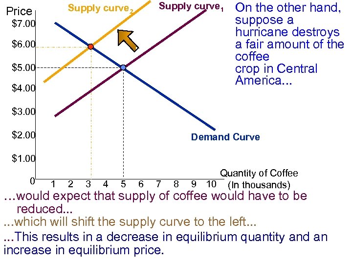
Supply curve 1 Supply curve 2 Price $7. 00 $6. 00 $5. 00 $4. 00 On the other hand, suppose a hurricane destroys a fair amount of the coffee crop in Central America. . . $3. 00 $2. 00 Demand Curve $1. 00 0 1 2 3 4 5 6 7 8 Quantity of Coffee 9 10 (In thousands) …would expect that supply of coffee would have to be reduced. . . which will shift the supply curve to the left. . . This results in a decrease in equilibrium quantity and an increase in equilibrium price.
The Great Tortilla Crises: • A sharp rise in the price of tortillas, a staple food of Mexico’s poor, which had gone from 25 cents a pound to between 35 and 45 cents a pound in just a few months in early 2007. Why were tortilla prices soaring? • It was a classic example of what happens to equilibrium prices when supply decreases. • Tortillas are made from corn; much of Mexico’s corn is imported from the United States, with the price of corn in both countries basically set in the U. S. corn market. • U. S. corn prices were rising rapidly thanks to surging demand in a new market: the market for ethanol. • This increase in the price of an input caused the supply of tortillas to decrease and equilibrium price to increase.
Other Examples Making predictions about price and quantity
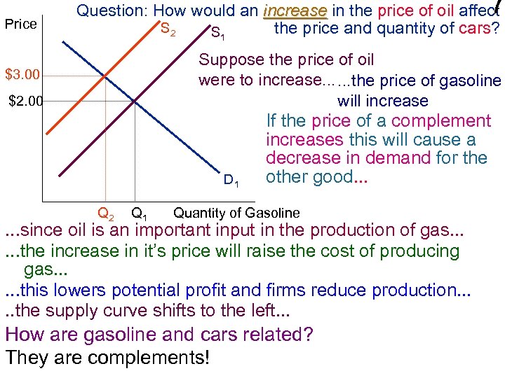
7 Price Question: How would an increase in the price of oil affect S 2 the price and quantity of cars? S 1 $3. 00 Suppose the price of oil were to increase. . . the price of gasoline will increase $2. 00 D 1 Q 2 Q 1 If the price of a complement increases this will cause a decrease in demand for the other good. . . Quantity of Gasoline . . . since oil is an important input in the production of gas. . . the increase in it’s price will raise the cost of producing gas. . . this lowers potential profit and firms reduce production. . . the supply curve shifts to the left. . . How are gasoline and cars related? They are complements!
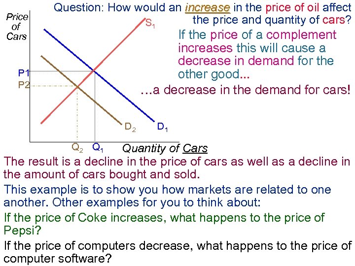
Price of Cars Question: How would an increase in the price of oil affect the price and quantity of cars? S 1 If the price of a complement increases this will cause a decrease in demand for the other good. . . …a decrease in the demand for cars! P 1 P 2 D 2 Q 1 D 1 Quantity of Cars The result is a decline in the price of cars as well as a decline in the amount of cars bought and sold. This example is to show you how markets are related to one another. Other examples for you to think about: If the price of Coke increases, what happens to the price of Pepsi? If the price of computers decrease, what happens to the price of computer software?
Example: Both Demand Supply curves shifting at the same time
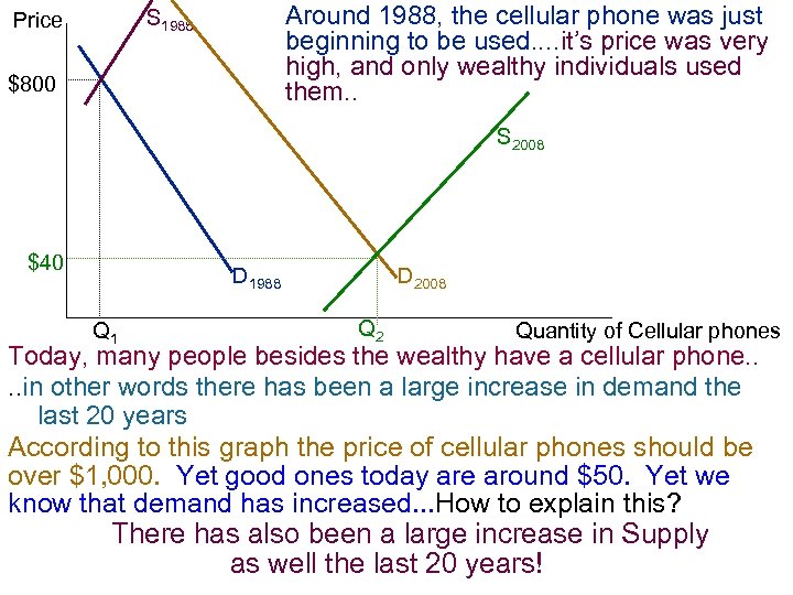
Around 1988, the cellular phone was just beginning to be used. . it’s price was very high, and only wealthy individuals used them. . S 1988 Price $800 S 2008 $40 D 1988 Q 1 D 2008 Q 2 Quantity of Cellular phones Today, many people besides the wealthy have a cellular phone. . in other words there has been a large increase in demand the last 20 years According to this graph the price of cellular phones should be over $1, 000. Yet good ones today are around $50. Yet we know that demand has increased. . . How to explain this? There has also been a large increase in Supply as well the last 20 years!
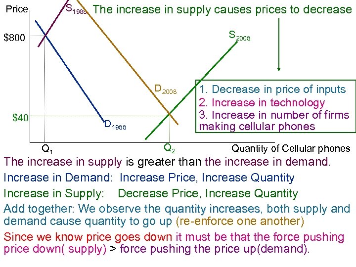
S 1988 Price The increase in supply causes prices to decrease S 2008 $800 D 2008 $40 1. Decrease in price of inputs 2. Increase in technology 3. Increase in number of firms making cellular phones Q 2 Quantity of Cellular phones D 1988 Q 1 The increase in supply is greater than the increase in demand. Increase in Demand: Increase Price, Increase Quantity Increase in Supply: Decrease Price, Increase Quantity Add together: We observe the quantity increases, both supply and increases demand cause quantity to go up (re-enforce one another) Since we know price goes down it must be that the force pushing price down( supply) > force pushing the price up(demand).
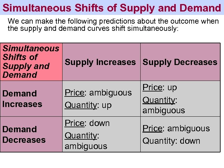
Simultaneous Shifts of Supply and Demand We can make the following predictions about the outcome when the supply and demand curves shift simultaneously: Simultaneous Shifts of Supply Increases Supply Decreases Supply and Demand Price: up Price: ambiguous Demand Quantity: Increases Quantity: up ambiguous Price: down Price: ambiguous Demand Quantity: Decreases Quantity: down ambiguous
Demand Supply Shifts at Work in the Global Economy • A recent drought in Australia reduced the amount of grass on which Australian dairy cows could feed, thus limiting the amount of milk these cows produced for export. • At the same time, a new tax levied by the government of Argentina raised the price of the milk the country exported, thereby decreasing Argentine milk sales worldwide. • These two developments produced a supply shortage in the world market, which dairy farmers in Europe couldn’t fill because of strict production quotas set by the European Union. • In China, meanwhile, demand for milk and milk products increased, as rising income levels drove higher per-capita consumption. • All these occurrences resulted in a strong upward pressure on the price of milk everywhere in 2007.
Summary 1. The supply and demand model illustrates how a competitive market works. 2. The demand schedule shows the quantity demanded at each price and is represented graphically by a demand curve. The law of demand says that demand curves slope downward. 3. A movement along the demand curve occurs when a price change leads to a change in the quantity demanded. When economists talk of increasing or decreasing demand, they mean shifts of the demand curve—a change in the quantity demanded at any given price.
Summary 4. There are five main factors that shift the demand curve: • A change in the prices of related goods or services • A change in income • A change in tastes • A change in expectations • A change in the number of consumers 5. The market demand curve for a good or service is the horizontal sum of the individual demand curves of all consumers in the market. 6. The supply schedule shows the quantity supplied at each price and is represented graphically by a supply curve. Supply curves usually slope upward.
Summary 7. A movement along the supply curve occurs when a price change leads to a change in the quantity supplied. When economists talk of increasing or decreasing supply, they mean shifts of the supply curve—a change in the quantity supplied at any given price. 8. There are five main factors that shift the supply curve: • A change in input prices • A change in the prices of related goods and services • A change in technology • A change in expectations • A change in the number of producers 9. The market supply curve for a good or service is the horizontal sum of the individual supply curves of all producers in the market.
Summary 10. The supply and demand model is based on the principle that the price in a market moves to its equilibrium price, or market-clearing price, the price at which the quantity demanded is equal to the quantity supplied. This quantity is the equilibrium quantity. When the price is above its market-clearing level, there is a surplus that pushes the price down. When the price is below its market-clearing level, there is a shortage that pushes the price up. 11. An increase in demand increases both the equilibrium price and the equilibrium quantity; a decrease in demand has the opposite effect. An increase in supply reduces the equilibrium price and increases the equilibrium quantity; a decrease in supply has the opposite effect. 12. Shifts of the demand curve and the supply curve can happen simultaneously.
517fd21fe444b7e2be0e971aba4dfcf0.ppt