Market Demand Supply Lecture 6 Dr Jennifer

Market Demand & Supply Lecture 6 Dr. Jennifer P. Wissink © 2018 John M. Abowd and Jennifer P. Wissink, all rights reserved. February 12, 2018

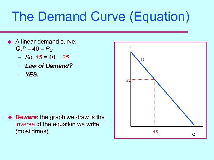The Demand Curve (Equation) u A linear demand curve: QXD = 40 – PX – So, 15 = 40 – 25 – Law of Demand? – YES. P D 25 u Beware: the graph we draw is the inverse of the equation we write (most times). 15 Q

The Demand Curve (Equation) u u Another example QD = 100 – 2 P P Q

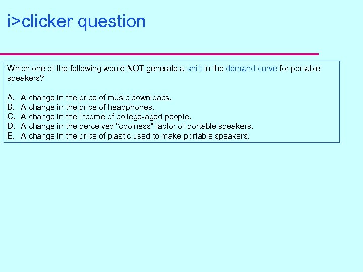i>clicker question Which one of the following would NOT generate a shift in the demand curve for portable speakers? A. B. C. D. E. A change in the price of music downloads. A change in the price of headphones. A change in the income of college-aged people. A change in the perceived “coolness” factor of portable speakers. A change in the price of plastic used to make portable speakers.

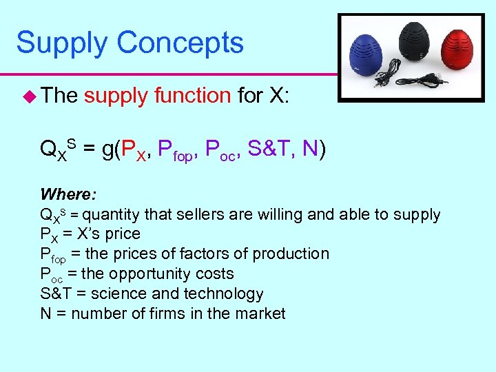Supply Concepts u The supply function for X: QXS = g(PX, Pfop, Poc, S&T, N) Where: QXS = quantity that sellers are willing and able to supply PX = X’s price Pfop = the prices of factors of production Poc = the opportunity costs S&T = science and technology N = number of firms in the market

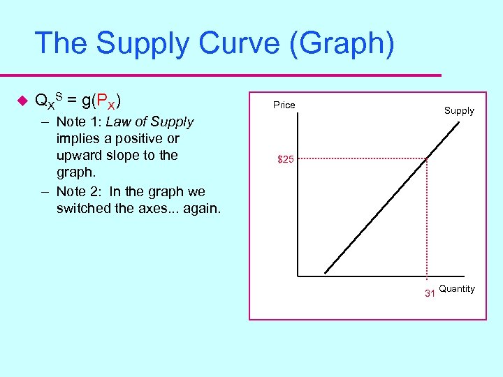The Supply Curve (Graph) u QXS = g(PX) – Note 1: Law of Supply implies a positive or upward slope to the graph. – Note 2: In the graph we switched the axes. . . again. Price Supply $25 31 Quantity

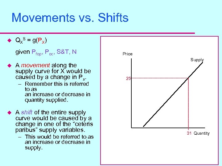Movements vs. Shifts u QXS = g(PX) given Pfop, Poc, S&T, N u A movement along the supply curve for X would be caused by a change in Px. – Remember this is referred to as an increase or decrease in quantity supplied. u A shift of the entire supply curve would be caused by a change in one of the “ceteris paribus” supply variables. – This would be referred to as an increase or decrease in supply. Price Supply 25 31 Quantity

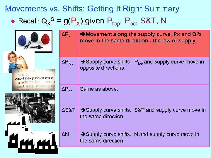Movements vs. Shifts: Getting It Right Summary u Recall: QXS = g(PX) given Pfop, Poc, S&T, N ΔPx Movement along the supply curve, Px and QSx move in the same direction - the law of supply. ΔPfop Supply curve shifts. Pfop and supply curve move in opposite directions. ΔPoc Same as above. ΔS&T Supply curve shifts. S&T and supply curve move in the same direction. ΔN Supply curve shifts. N and supply curve move in the same direction.

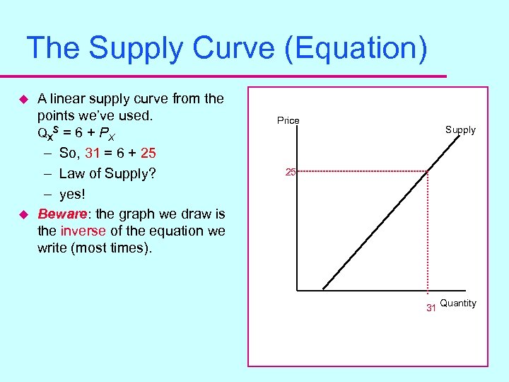The Supply Curve (Equation) u u A linear supply curve from the points we’ve used. QXS = 6 + PX – So, 31 = 6 + 25 – Law of Supply? – yes! Beware: the graph we draw is the inverse of the equation we write (most times). Price Supply 25 31 Quantity

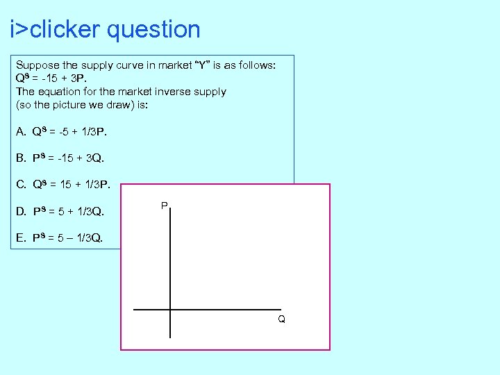i>clicker question Suppose the supply curve in market “Y” is as follows: QS = -15 + 3 P. The equation for the market inverse supply (so the picture we draw) is: A. QS = -5 + 1/3 P. B. PS = -15 + 3 Q. C. QS = 15 + 1/3 P. D. PS = 5 + 1/3 Q. P E. PS = 5 – 1/3 Q. Q

Market Equilibrium u We are considering the market for portable speakers. u Recall that we defined the following for our market: – The type and style of portable speakers. – The quality of the portable speakers. – All other attributes of the generic portable speaker. – A time frame that applies to our market for portable speakers. u Demanders are the buyers and from them we get the demand function, etc. – Qx. D = f(PX, Ps, Pc, I, T&P, Pop) u Suppliers are the sellers and from them we get the supply function, etc. – QXS = g(PX, Pfop, Poc, S&T, N) u The market is a perfectly competitive market.

Market Equilibrium (Verbal) u. A place of “rest”. u Equilibrium: a price where the quantity demanded equals the quantity supplied. u In notation: – Find a PX* so that: QXD(PX*) = QXS(PX*)

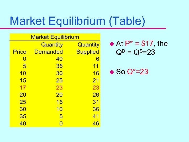Market Equilibrium (Table) u At P* = $17, the QD = QS=23 u So Q*=23

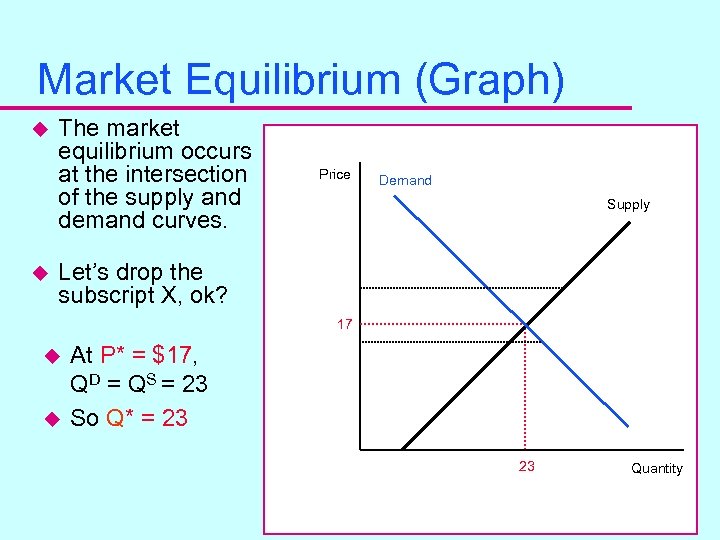Market Equilibrium (Graph) u u The market equilibrium occurs at the intersection of the supply and demand curves. Price Demand Supply Let’s drop the subscript X, ok? 17 u u At P* = $17, QD = QS = 23 So Q* = 23 23 Quantity

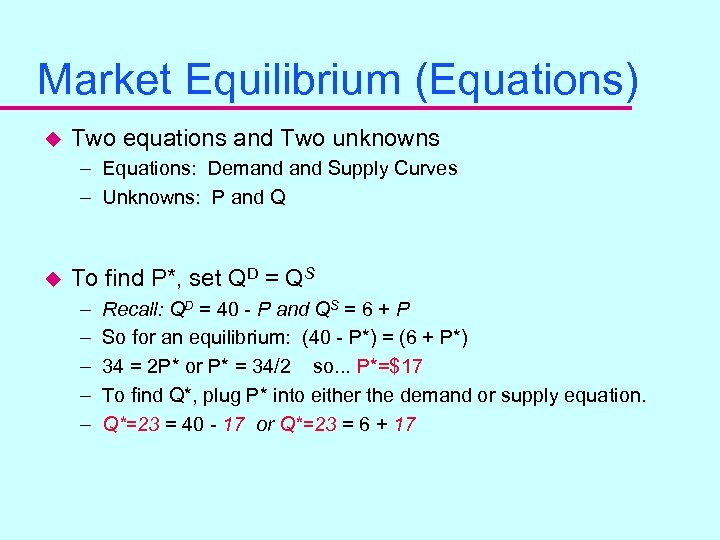Market Equilibrium (Equations) u Two equations and Two unknowns – Equations: Demand Supply Curves – Unknowns: P and Q u To find P*, set QD = QS – – – Recall: QD = 40 - P and QS = 6 + P So for an equilibrium: (40 - P*) = (6 + P*) 34 = 2 P* or P* = 34/2 so. . . P*=$17 To find Q*, plug P* into either the demand or supply equation. Q*=23 = 40 - 17 or Q*=23 = 6 + 17

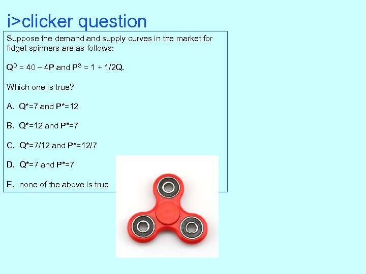i>clicker question Suppose the demand supply curves in the market for fidget spinners are as follows: QD = 40 – 4 P and PS = 1 + 1/2 Q. Which one is true? A. Q*=7 and P*=12 B. Q*=12 and P*=7 C. Q*=7/12 and P*=12/7 D. Q*=7 and P*=7 E. none of the above is true

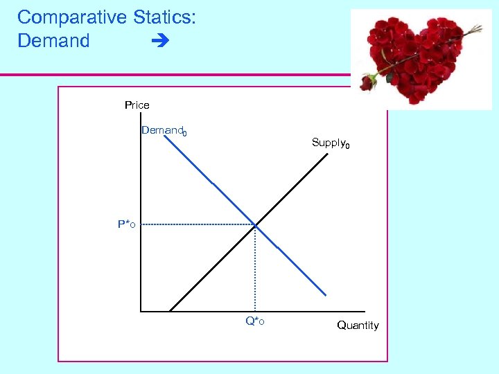
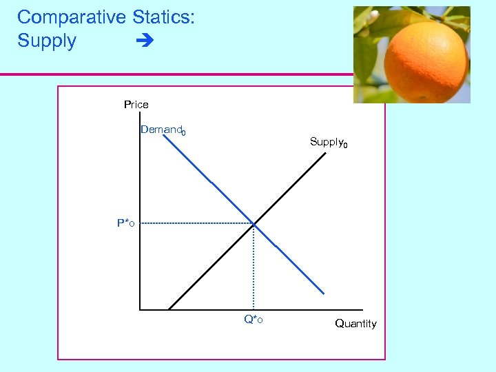
Now What? Comparative Statics! u u u SIMPLE AS THAT!? Then what. . Use the model to make predictions. Something changes in the market. – – u u u Something that changes Demand. Something that changes Supply. Something that changes both! Something the government does to prevent an equilibrium. Would get a new equilibrium. Compare one market equilibrium with another market equilibrium and see what happens to P* and Q*. Compare two equilibriums - compare two static situations - comparative statics!

The Roses Market u u What impact will the approaching holiday have on the cut roses market? What do you predict will happen to the equilibrium market price and quantity?

Comparative Statics: Demand Price Demand 0 Supply 0 P*o Quantity

The Florida Orange Market u Number Crunch in Latest Florida Orange Crop Estimate (2/8/2018) – – u http: //www. growingproduce. com/citrus/numbers-crunch-latest-florida-orange-crop-estimate/ Forecasters from USDA are trying to take all factors into account. The agency’s updated 2017 -2018 Florida allorange crop estimate now stands at 45 million boxes, down 1 million boxes from last month’s estimate and 35% off last season’s tally. What do you predict will happen to the equilibrium market price and quantity?

Comparative Statics: Supply Price Demand 0 Supply 0 P*o Quantity