Mar 19, 2016 11 Probability Theory

Mar 19, 2016 11 Probability Theory And Statistics The Course of Lectures. Lecture

Mar 19, 2016 2 Lecture 9 Uniform Distribution. Normal (Gaussian Distribution) Distributions.

Mar 19, 2016 3 Contents Uniform distribution – the general view The Normal Distribution

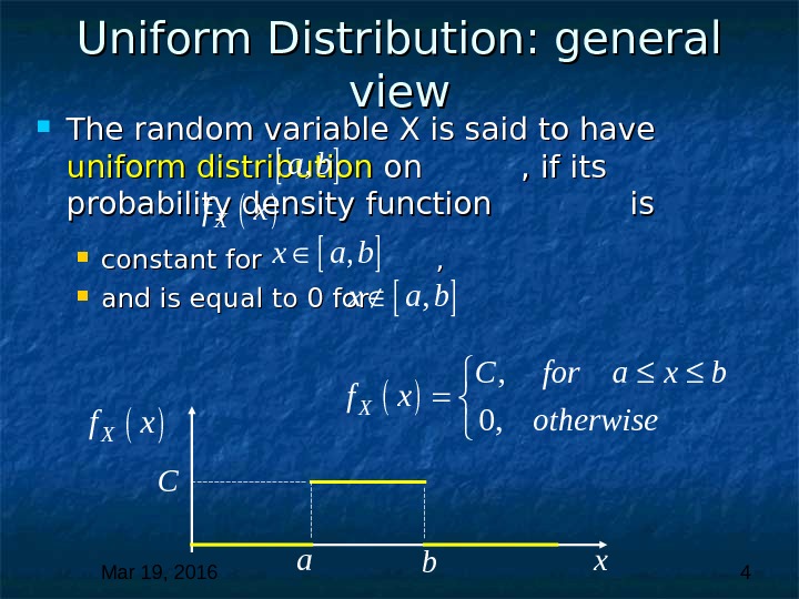
Mar 19, 2016 4 Uniform Distribution: general view The random variable X is said to have uniform distribution on , if its probability density function is constant for , , and is equal to 0 for Xf x , a b , x a b Xf x b ax C , 0, X C for a x b f x otherwise

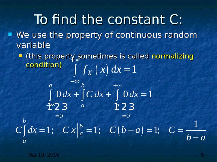
Mar 19, 2016 5 To find the constant C: We use the property of continuous random variable (this property sometimes is called normalizing condition) 1 1; 1; 1; b b a a. C dx C b a 1 Xf x dx 00 0 0 1 a b dx C dx dx

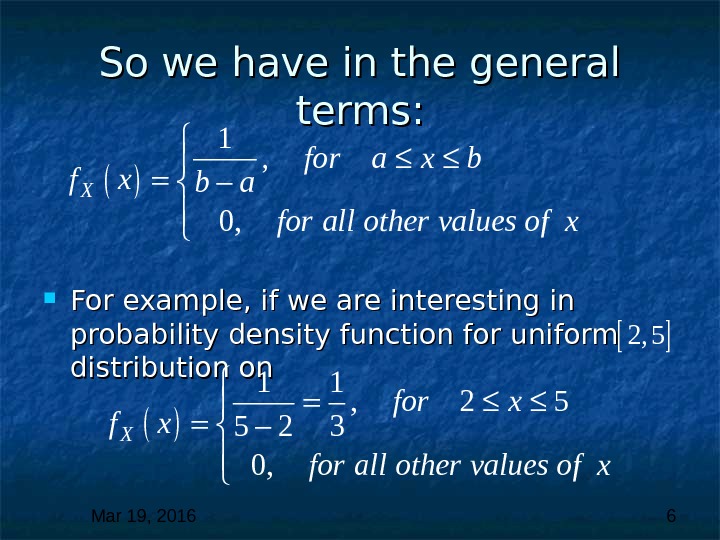
Mar 19, 2016 6 So we have in the general terms: For example, if we are interesting in probability density function for uniform distribution on 1 , 0, X for a x b f x b a for all other values of x 2, 5 1 1 , 2 5 5 2 3 0, X for x for all other values of x

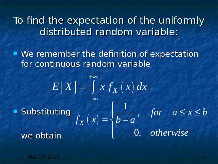
Mar 19, 2016 7 To find the expectation of the uniformly distributed random variable: We remember the definition of expectation for continuous random variable Substituting we obtain XE X x f x dx 1 , 0, X for a x b f x b a otherwise

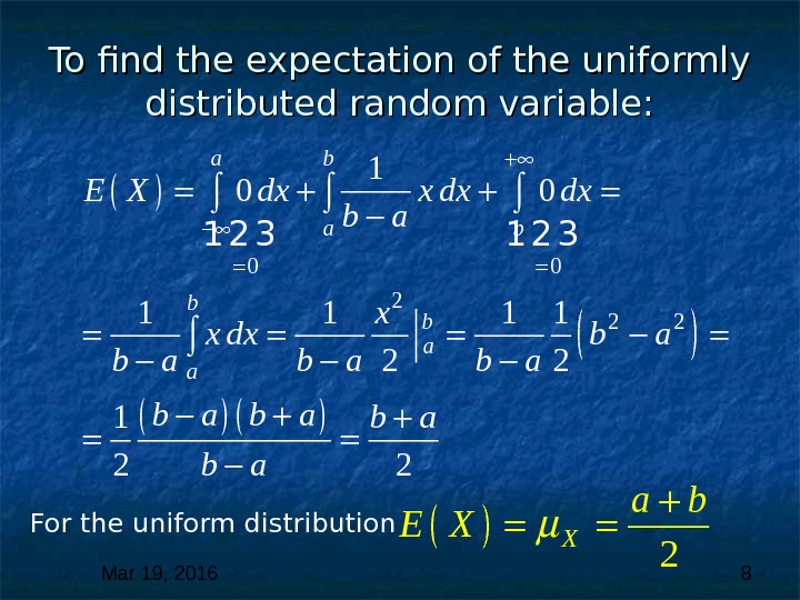
Mar 19, 2016 8 To find the expectation of the uniformly distributed random variable: 0 0 2 2 21 0 0 1 1 2 2 a b b b a a. E X dx x dx dx b a x x dx b a b a 1 2 3 2 X a b E X For the uniform distribution

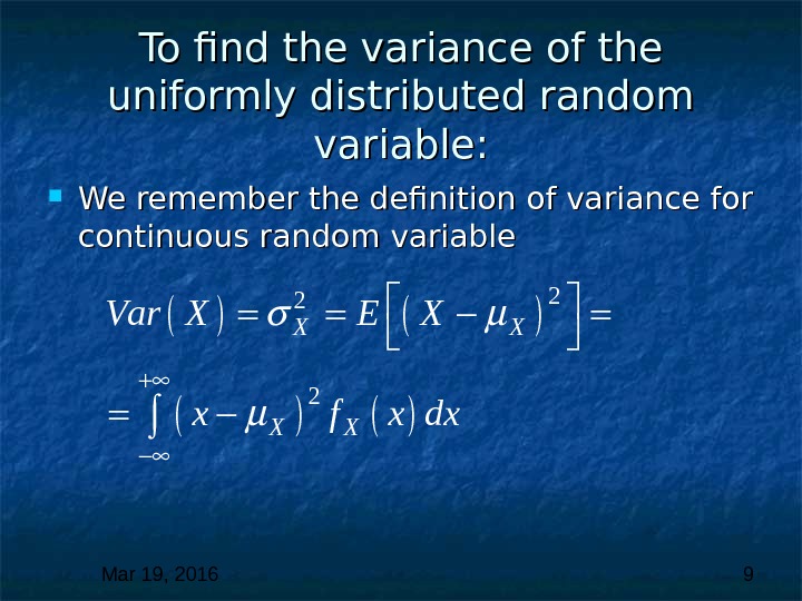
Mar 19, 2016 9 To find the variance of the uniformly distributed random variable: We remember the definition of variance for continuous random variable 2 2 2 X X Var X E X x f x dx

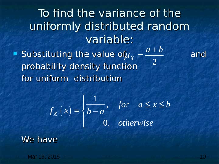
Mar 19, 2016 10 To find the variance of the uniformly distributed random variable: Substituting the value of and probability density function for uniform distribution We have 2 X a b 1 , 0, X for a x b f x b a otherwise

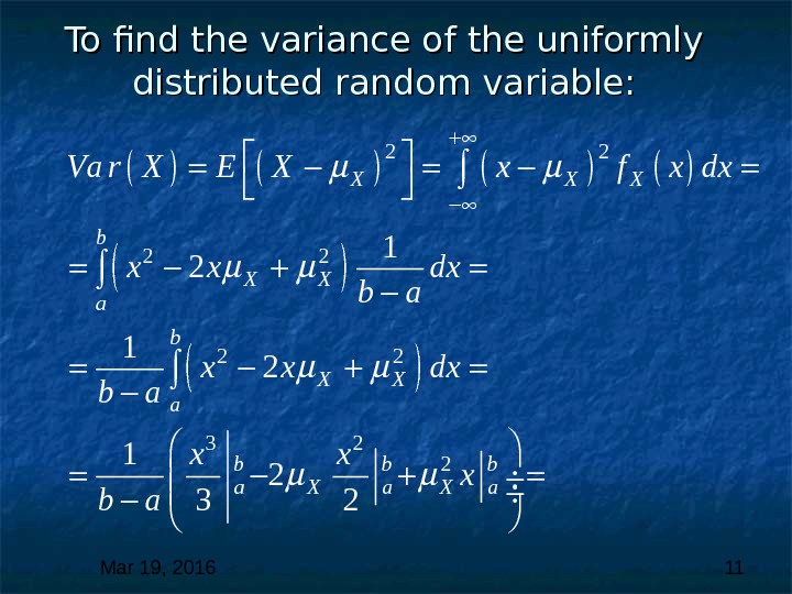
Mar 19, 2016 11 To find the variance of the uniformly distributed random variable: 2 2 2 3 2 21 2 1 2 3 2 X X X b X X a b b b a X a. Va r X E X x f x dx x x dx b a x x x b a

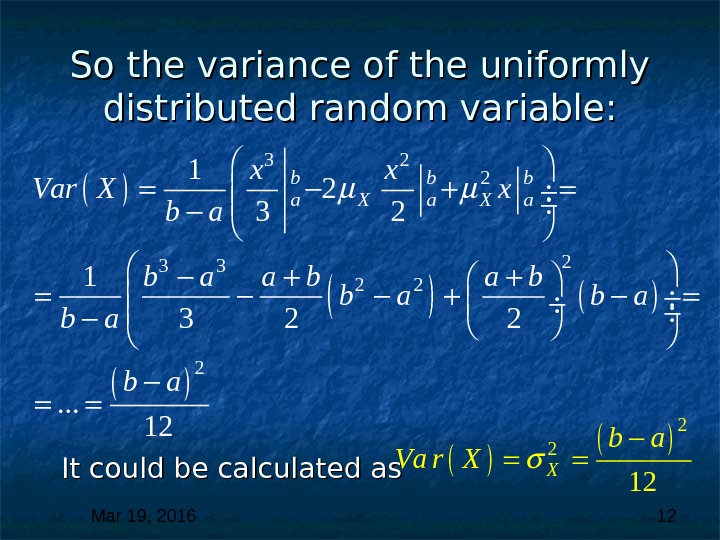
Mar 19, 2016 12 So the variance of the uniformly distributed random variable: It could be calculated as 2 2 12 X b a Va r X 3 2 2 2 3 3 2 2 2 1 2 3 2 1 3 2 2. . . 12 b b b a X a x x Var X x b a a b b a b a

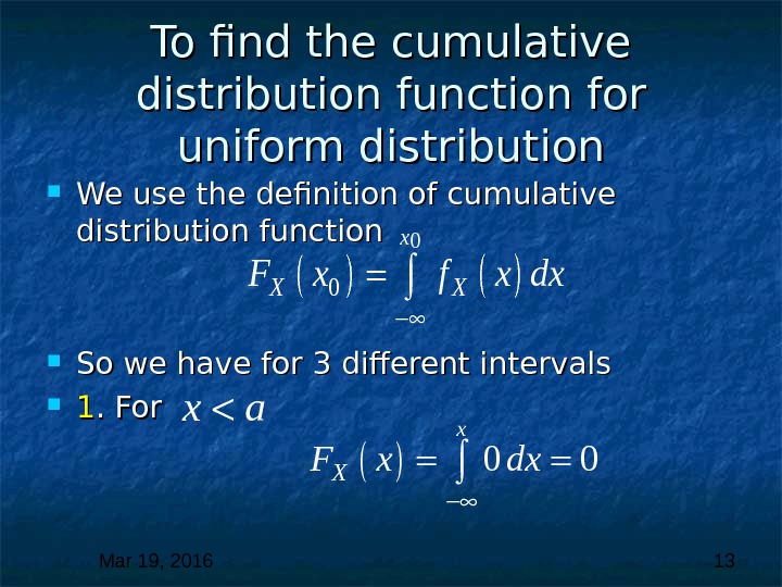
Mar 19, 2016 13 To find the cumulative distribution function for uniform distribution We use the definition of cumulative distribution function So we have for 3 different intervals 11. For 0 0 x XF x dx x a 0 0 x X XF x f x dx

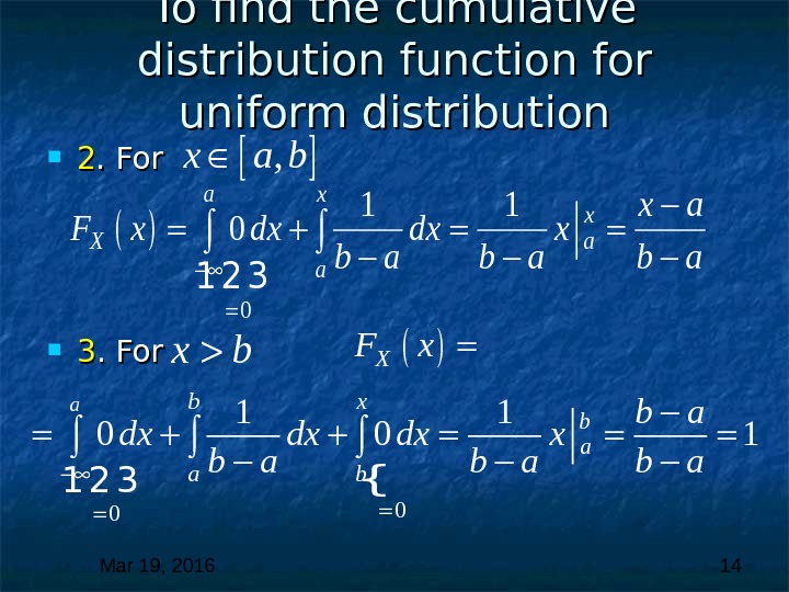
Mar 19, 2016 14 To find the cumulative distribution function for uniform distribution 22. For 33. For , x a b { 0 0 1 1 0 0 1 a X b x b a a b F x b a dx dx dx x b a b a 1 2 3 0 1 1 0 a x x X a a x a F x dx dx x b a b a 1 2 3 x b

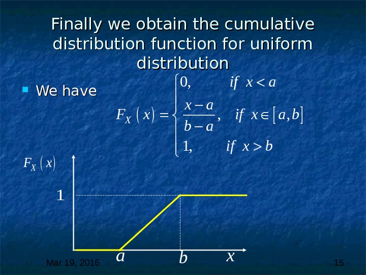
Mar 19, 2016 15 Finally we obtain the cumulative distribution function for uniform distribution We have 0, , , 1, X if x a F x if x a b b a if x b XF x x ba

Mar 19, 2016 16 The Normal Distribution We introduce now a continuous distribution that plays a central role in a very large body of statistical analysis. . For example, suppose that a big group of students takes a test. A large proportion of their scores are likely to be concentrated about the mean, and the numbers of scores in ranges of a fixed width are likely to «tail off” away from the mean.

Mar 19, 2016 17 The Normal Distribution If the average score on the test is 60, we would expect to find, for instance, more students with scores in the range 55 -65 than in the range 85 -95 These considerations suggest a probability density function that peaks at the mean and tails off at its extremities. One distribution with these properties is the normal distribution , , whose probability density function is shown below. As can be see this density function is bell-shaped.

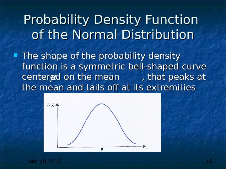
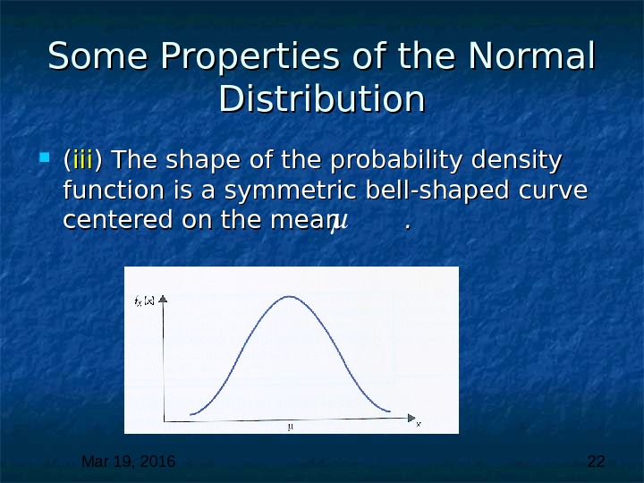
Mar 19, 2016 18 Probability Density Function of the Normal Distribution The shape of the probability density function is a symmetric bell-shaped curve centered on the mean , that peaks at the mean and tails off at its extremities

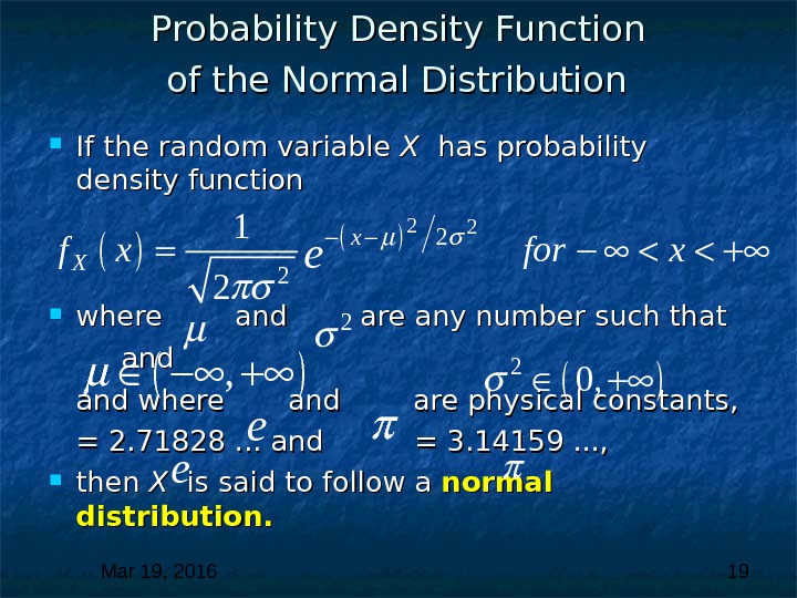
Mar 19, 2016 19 Probability Density Function of the Normal Distribution If the random variable X X has probability density function where and are any number such that andand where and are physical constants, = 2. 71828. . . and = 3. 14159. . . , then X X is said to follow a normal distribution. 22 2 21 2 x Xf x for x e e , 2 20, e

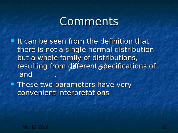
Mar 19, 2016 20 Comments It can be seen from the definition that there is not a single normal distribution but a whole family of distributions, resulting from different specifications of and . . These two parameters have very convenient interpretations

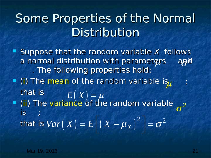
Mar 19, 2016 21 Some Properties of the Normal Distribution Suppose that the random variable X X follows a normal distribution with parameters and . . The following properties hold: (( ii ) The mean of the random variable is ; that is (( iiii ) The variance of the random variable is is ; ; that is 22 XVar X E X 2 E X

Mar 19, 2016 22 Some Properties of the Normal Distribution (( iiiiii ) The shape of the probability density function is a symmetric bell-shaped curve centered on the mean . .

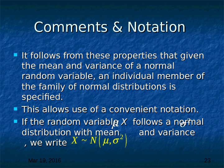
Mar 19, 2016 23 Comments & Notation It follows from these properties that given the mean and variance of a normal random variable, an individual member of the family of normal distributions is specified. This allows use of a convenient notation. If the random variable X X follows a normal distribution with mean and variance , , we write 2 2 ~ , X N

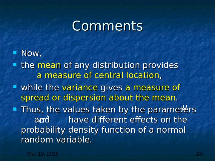
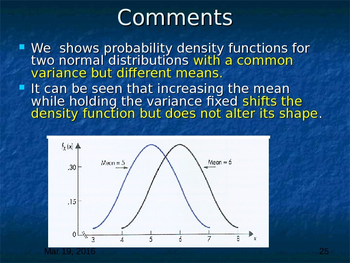
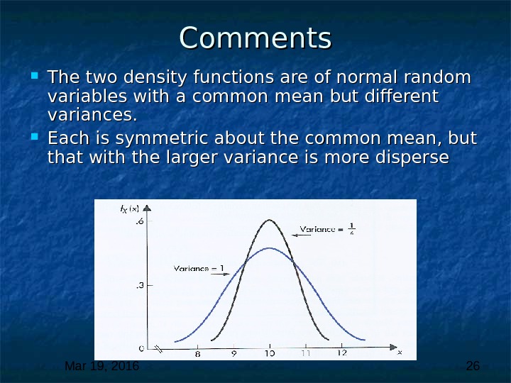
Mar 19, 2016 24 Comments Now, the mean of any distribution provides a measure of central location , , while the variance gives a measure of spread or dispersion about the mean. . Thus, the values taken by the parameters and have different effects on the probability density function of a normal random variable.

Mar 19, 2016 25 Comments We shows probability density functions for two normal distributions with a common variance but different means. It can be seen that increasing the mean while holding the variance fixed shifts the density function but does not alter its shape. .

Mar 19, 2016 26 Comments The two density functions are of normal random variables with a common mean but different variances. Each is symmetric about the common mean, but that with the larger variance is more disperse

Mar 19, 2016 27 Cumulative Distribution Function of the Normal Distribution An extremely important practical question concerns the determination of probabilities from a specified normal distribution. As a first step in determining probabilities, we introduce the cumulative distribution function

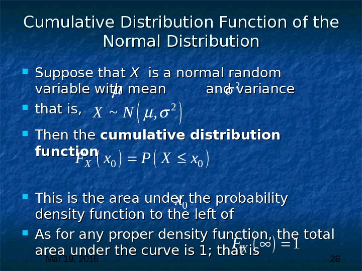
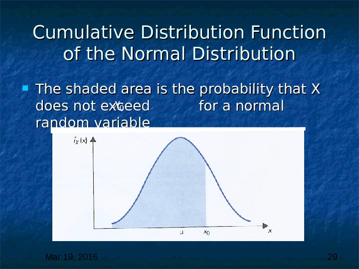
Mar 19, 2016 28 Cumulative Distribution Function of the Normal Distribution Suppose that X X is a normal random variable with mean and variance that is, Then the cumulative distribution function This is the area under the probability density function to the left of As for any proper density function, the total area under the curve is 1; that is 2 2 ~ , X N 0 0 XF x P X x 0 x 1 X

Mar 19, 2016 29 Cumulative Distribution Function of the Normal Distribution The shaded area is the probability that X does not exceed for a normal random variable 0 x

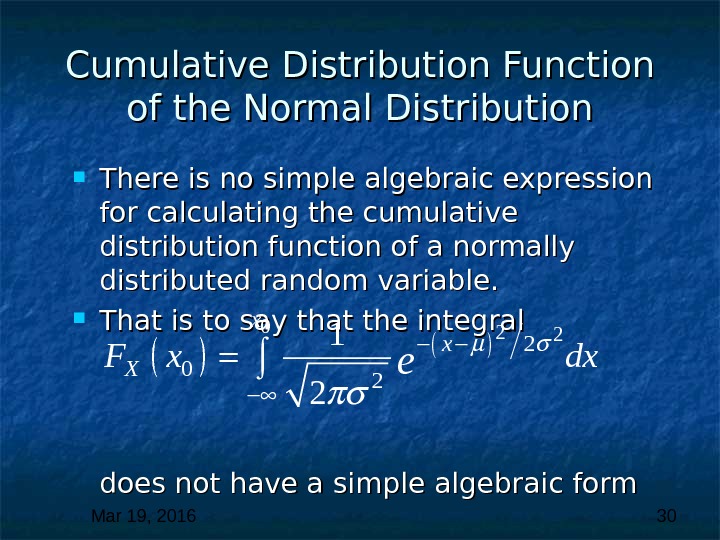
Mar 19, 2016 30 Cumulative Distribution Function of the Normal Distribution There is no simple algebraic expression for calculating the cumulative distribution function of a normally distributed random variable. That is to say that the integral does not have a simple algebraic form 022 2 0 2 1 2 x x XF x dxe

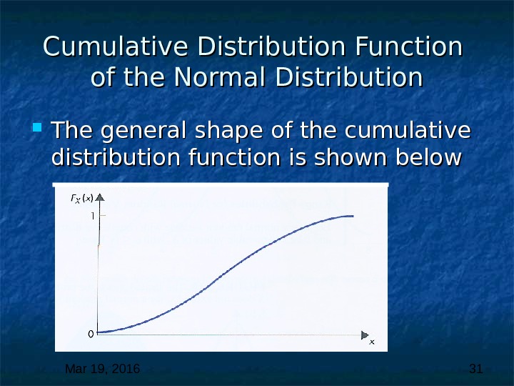
Mar 19, 2016 31 Cumulative Distribution Function of the Normal Distribution The general shape of the cumulative distribution function is shown below

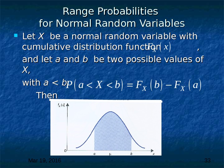
Mar 19, 2016 32 Range Probabilities for Normal Random Variables We have already seen that for any continuous random variable, probabilities can be expressed in terms of the cumulative distribution function

Mar 19, 2016 33 Range Probabilities for Normal Random Variables Let X X be a normal random variable with cumulative distribution function , , and let a a and b b be two possible values of X, X, with a < b. Then. X XP a X b F a XF x

Mar 19, 2016 34 Range Probabilities for Normal Random Variables Any required probability can be obtained from the cumulative distribution function. However, a crucial difficulty remains because there does not exist a convenient formula for determining the cumulative distribution function. . In principle, for any specific normal distribution, probabilities could be obtained by numerical methods using an electronic computer.

Mar 19, 2016 35 Range Probabilities for Normal Random Variables However, it would be enormously tedious if we had to carry out such an operation for every normal distribution we encountered. Fortunately, probabilities for any normal distribution can always be expressed in terms of probabilities for a single normal distribution for which the cumulative distribution function has been evaluated and tabulated.

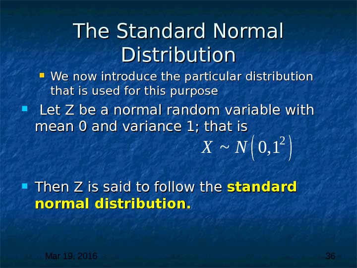
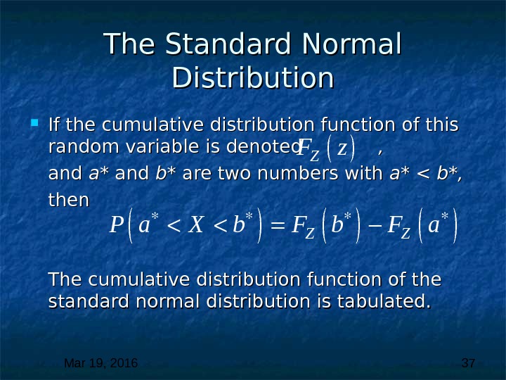
Mar 19, 2016 36 The Standard Normal Distribution We now introduce the particular distribution that is used for this purpose Let Z be a normal random variable with mean 0 and variance 1; that is Then Z is said to follow the standard normal distribution. 2~ 0, 1 X N

Mar 19, 2016 37 The Standard Normal Distribution If the cumulative distribution function of this random variable is denoted , , and a* a* and b* b* are two numbers with a* < b*, then The cumulative distribution function of the standard normal distribution is tabulated. ZF z Z ZP a X b F a

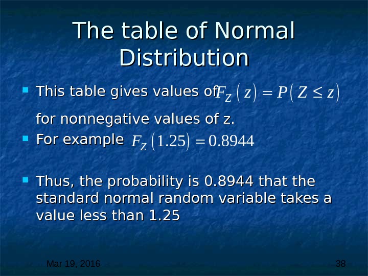
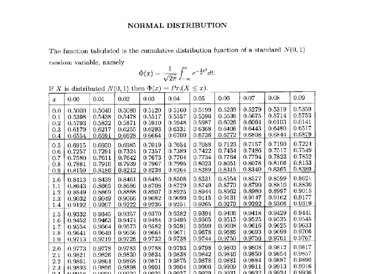
Mar 19, 2016 38 The table of Normal Distribution This table gives values of for nonnegative values of z. For example Thus, the probability is 0. 8944 that the standard normal random variable takes a value less than 1. 25 ZF z P Z z 1. 25 0. 8944 Z

Mar 19,

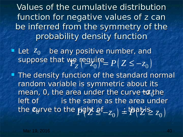
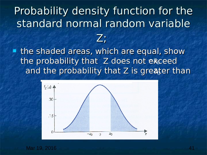
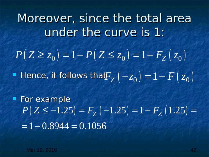
Mar 19, 2016 40 Values of the cumulative distribution function for negative values of z can be inferred from the symmetry of the probability density function Let be any positive number, and suppose that we require The density function of the standard normal random variable is symmetric about its mean, 0, the area under the curve to the left of is the same as the area under the curve to the right of ; that is 0 0 P Z z 0 0 ZF z P Z z 0 z 0 z

Mar 19, 2016 41 Probability density function for the standard normal random variable Z; Z; the shaded areas, which are equal, show the probability that Z does not exceed and the probability that Z is greater than 0 z 0 z

Mar 19, 2016 42 Moreover, since the total area under the curve is 1: Hence, it follows that For example 0 0 1 ZF z 0 0 01 1 ZP Z z F z 1. 25 1 0. 8944 0. 1056 Z ZP Z

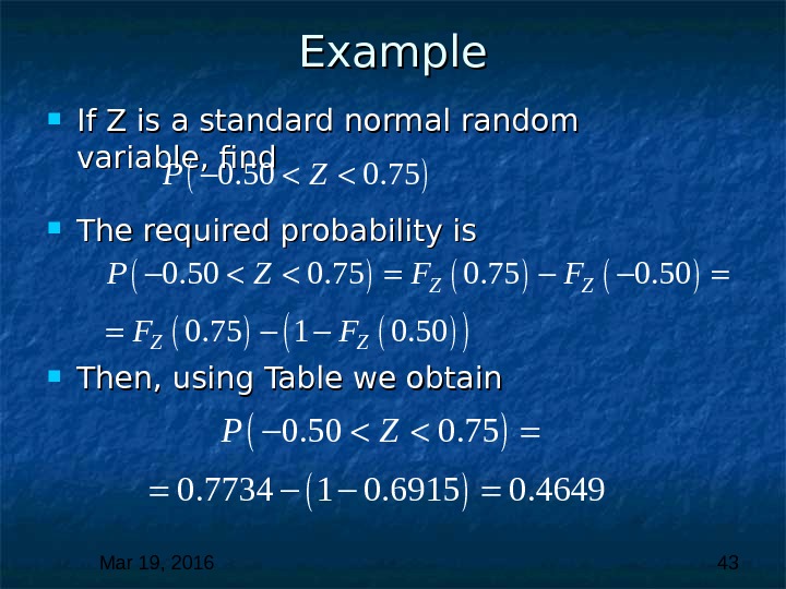
Mar 19, 2016 43 Example If Z is a standard normal random variable, find The required probability is Then, using Table we obtain 0. 50 0. 75 1 0. 50 Z Z P Z F F 0. 50 0. 75 P Z 0. 50 0. 75 0. 7734 1 0. 6915 0. 4649 P Z

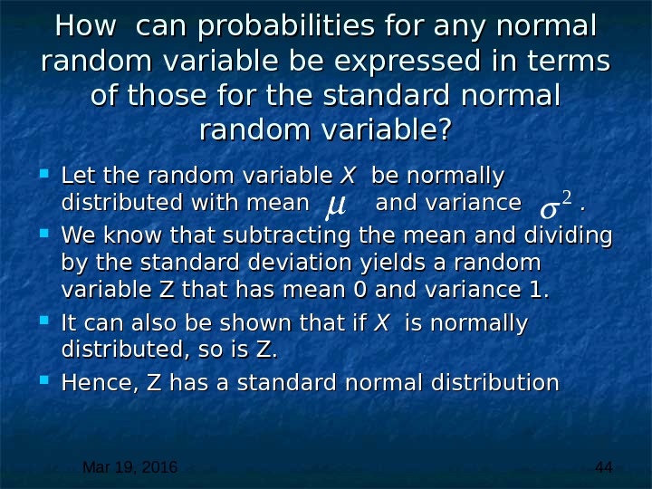
Mar 19, 2016 44 How can probabilities for any normal random variable be expressed in terms of those for the standard normal random variable? Let the random variable X X be normally distributed with mean and variance . . We know that subtracting the mean and dividing by the standard deviation yields a random variable Z that has mean 0 and variance 1. It can also be shown that if X X is normally distributed, so is Z. Hence, Z has a standard normal distribution

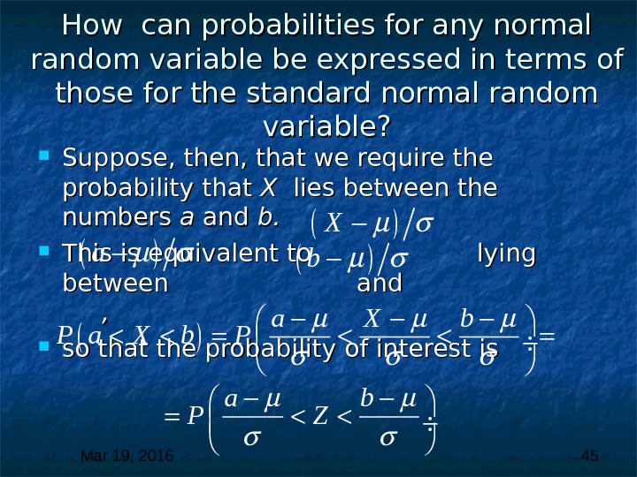
Mar 19, 2016 45 How can probabilities for any normal random variable be expressed in terms of those for the standard normal random variable? Suppose, then, that we require the probability that X X lies between the numbers a a and b. b. This is equivalent to lying between and , , so that the probability of interest is. X a X b P a b P Z b a

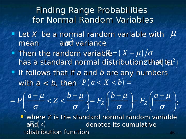
Mar 19, 2016 46 Finding Range Probabilities for Normal Random Variables Let X X be a normal random variable with mean and variance Then the random variable has a standard normal distribution; that is, It follows that if a a and b b are any numbers with a < b, then where Z is the standard normal random variable and denotes its cumulative distribution function ZF z Z ZP a X b a b b a P Z F F 2 Z X 2 ~ 0, 1 Z N

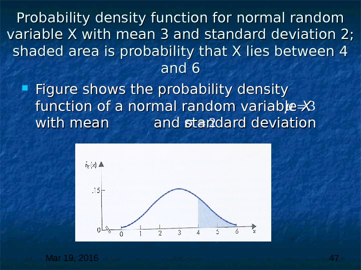
Mar 19, 2016 47 Probability density function for normal random variable X with mean 3 and standard deviation 2; shaded area is probability that X lies between 4 and 6 Figure shows the probability density function of a normal random variable X X with mean and standard deviation

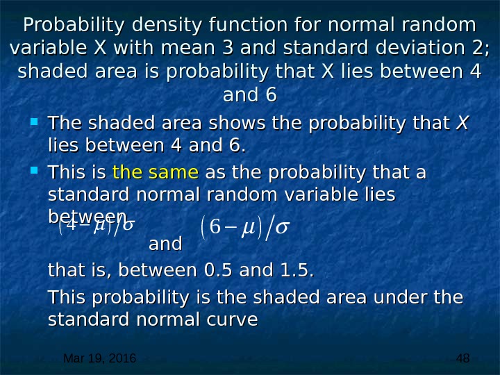
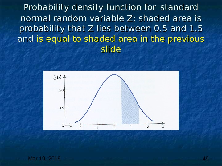
Mar 19, 2016 48 Probability density function for normal random variable X with mean 3 and standard deviation 2; shaded area is probability that X lies between 4 and 6 The shaded area shows the probability that X X lies between 4 and 6. This is the same as the probability that a standard normal random variable lies between andand that is, between 0. 5 and 1. 5. This probability is the shaded area under the standard normal curve

Mar 19, 2016 49 Probability density function for standard normal random variable Z; shaded area is probability that Z lies between 0. 5 and 1. 5 and is equal to shaded area in the previous slide

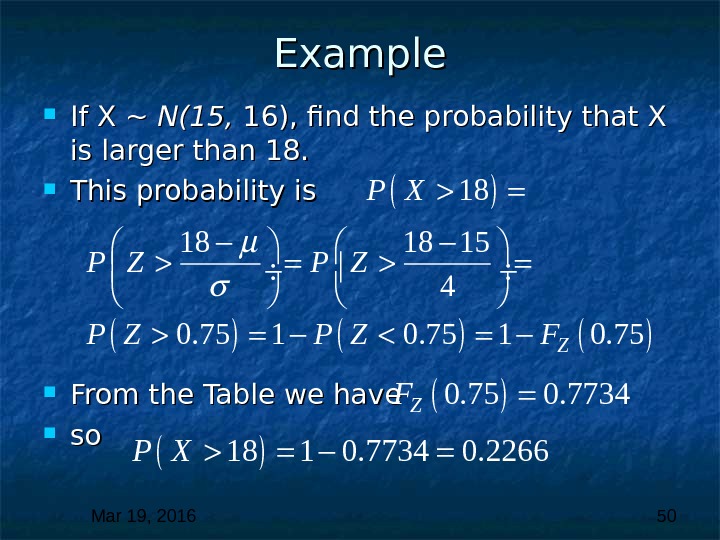
Mar 19, 2016 50 Example If X ~ N(15, 16), find the probability that X is larger than 18. This probability is From the Table we have so so 18 1 0. 7734 0. 2266 P X 0. 75 0. 7734 ZF 18 18 18 15 4 0. 75 1 0. 75 Z P X P Z P Z

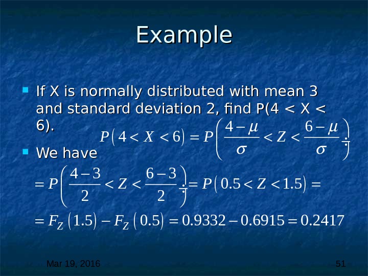
Mar 19, 2016 51 Example If X is normally distributed with mean 3 and standard deviation 2, find P(4 < X < 6). We have 4 6 4 3 6 3 0. 5 1. 5 2 2 1. 5 0. 9332 0. 6915 0. 2417 Z Z P X P Z P Z

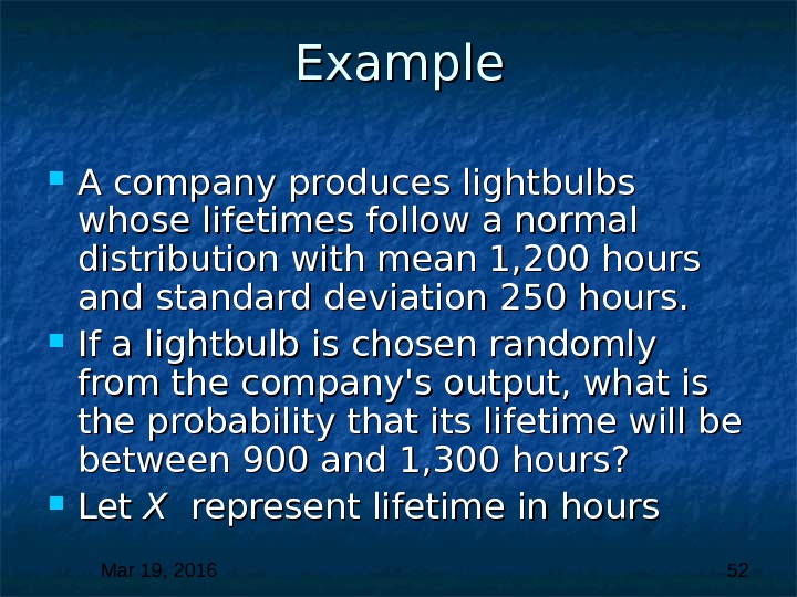
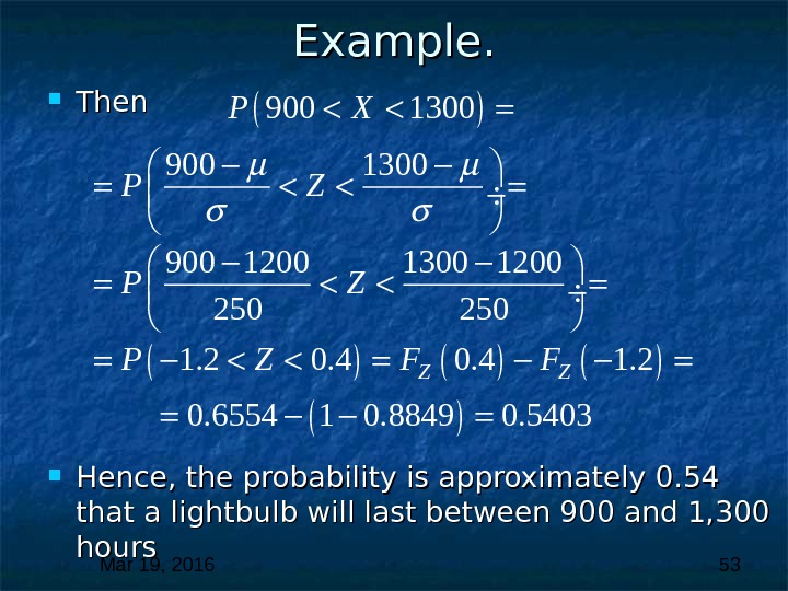
Mar 19, 2016 52 Example A company produces lightbulbs whose lifetimes follow a normal distribution with mean 1, 200 hours and standard deviation 250 hours. If a lightbulb is chosen randomly from the company’s output, what is the probability that its lifetime will be between 900 and 1, 300 hours? Let X X represent lifetime in hours

Mar 19, 2016 53 Example. Then Hence, the probability is approximately 0. 54 that a lightbulb will last between 900 and 1, 300 hours 900 1300 900 1200 1300 1200 250 1. 2 0. 4 1. 2 0. 6554 1 0. 8849 0. 5403 Z Z P X P Z P Z

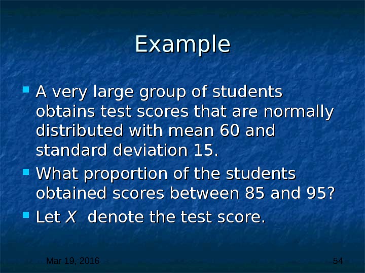
Mar 19, 2016 54 Example A very large group of students obtains test scores that are normally distributed with mean 60 and standard deviation 15. What proportion of the students obtained scores between 85 and 95? Let X X denote the test score.

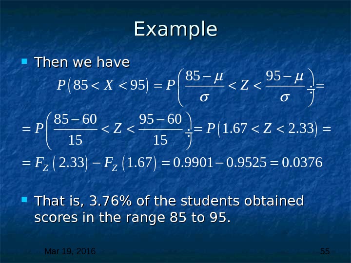
Mar 19, 2016 55 Example Then we have That is, 3. 76% of the students obtained scores in the range 85 to 95. 85 95 85 60 95 60 1. 67 2. 33 15 15 2. 33 1. 67 0. 9901 0. 9525 0. 0376 Z Z P X P Z P Z

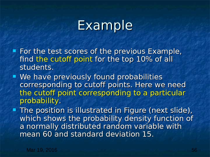
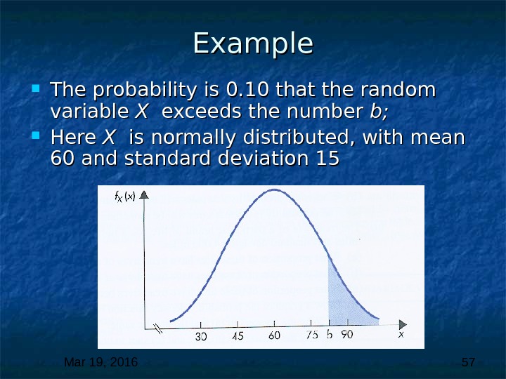
Mar 19, 2016 56 Example For the test scores of the previous Example, find the cutoff point for the top 10% of all students. We have previously found probabilities corresponding to cutoff points. Here we need the cutoff point corresponding to a particular probability. . The position is illustrated in Figure (next slide), which shows the probability density function of a normally distributed random variable with mean 60 and standard deviation 15.

Mar 19, 2016 57 Example The probability is 0. 10 that the random variable X X exceeds the number b; b; Here X X is normally distributed, with mean 60 and standard deviation

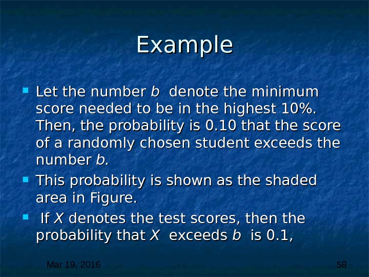
Mar 19, 2016 58 Example Let the number b b denote the minimum score needed to be in the highest 10%. Then, the probability is 0. 10 that the score of a randomly chosen student exceeds the number b. b. This probability is shown as the shaded area in Figure. If If X X denotes the test scores, then the probability that X X exceeds b b is 0. 1,

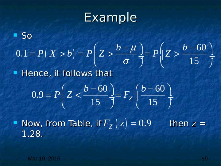
Mar 19, 2016 59 Example So. So Hence, it follows that Now, from Table, if then z = 1. 28. 60 0. 1 15 b b P X b P Z 60 60 0. 9 15 15 Z b b P Z F 0. 9 ZF z

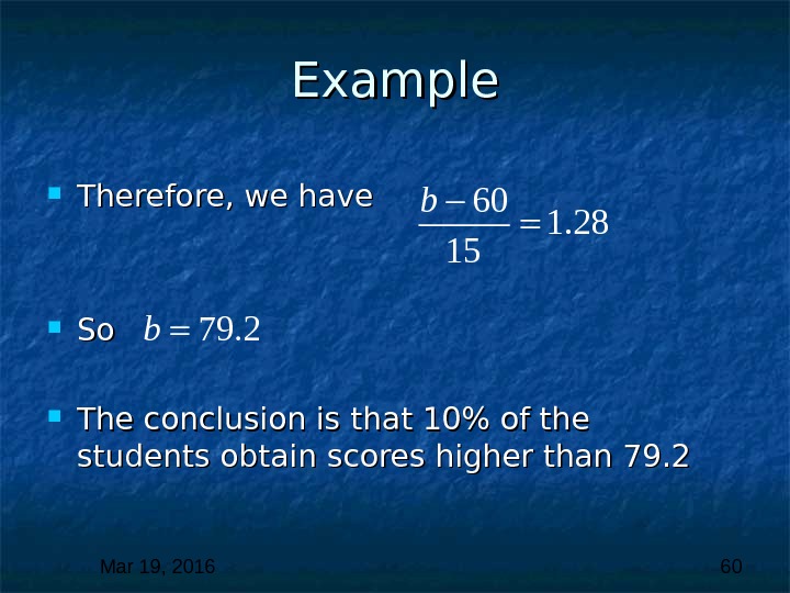
Mar 19, 2016 60 Example Therefore, we have So. So The conclusion is that 10% of the students obtain scores higher than 79. 2 60 1. 28 15 b 79. 2 b

Mar 19, 2016 61 Comments In Examples, if the scores awarded on the test were integers, the distribution of scores would be inherently discrete. Nevertheless, the normal distribution can typically provide an adequate approximation in such circumstances. We will see later that the normal distribution can often be employed as an approximation to discrete distributions. As a preliminary, we introduce in the next lecture a result that provides strong justification for the emphasis given to the normal distribution.

Mar 19, 2016 62 Thank you for your attention!