Managing Flow Variability Safety Inventory 1 Operations Management

Managing Flow Variability: Safety Inventory 1 Operations Management Session 23: Newsvendor Model

Managing Flow Variability: Safety Inventory Uncertain Demand 2 Uncertain Demand: What are the relevant trade-offs? – Overstock • Demand is lower than the available inventory • Inventory holding cost – Understock • Shortage- Demand is higher than the available inventory – Why do we have shortages? – What is the effect of shortages? Session 23 Operations Management 2

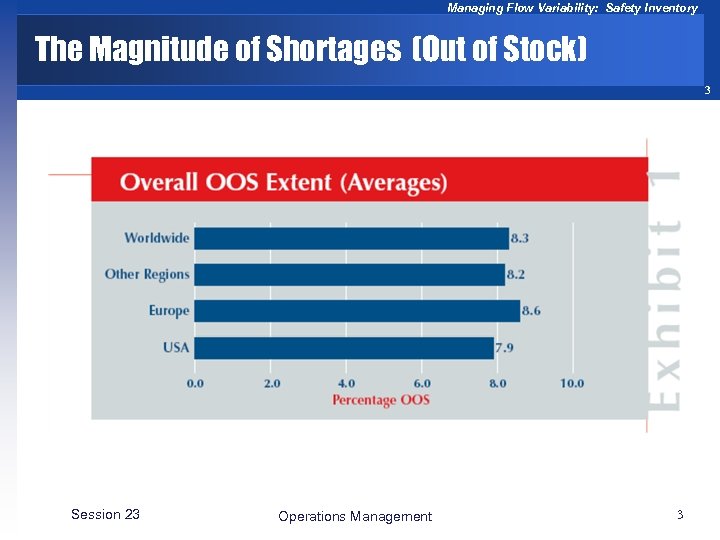
Managing Flow Variability: Safety Inventory The Magnitude of Shortages (Out of Stock) 3 Session 23 Operations Management 3

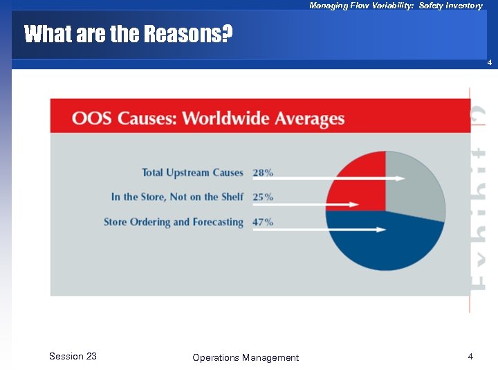
Managing Flow Variability: Safety Inventory What are the Reasons? 4 Session 23 Operations Management 4

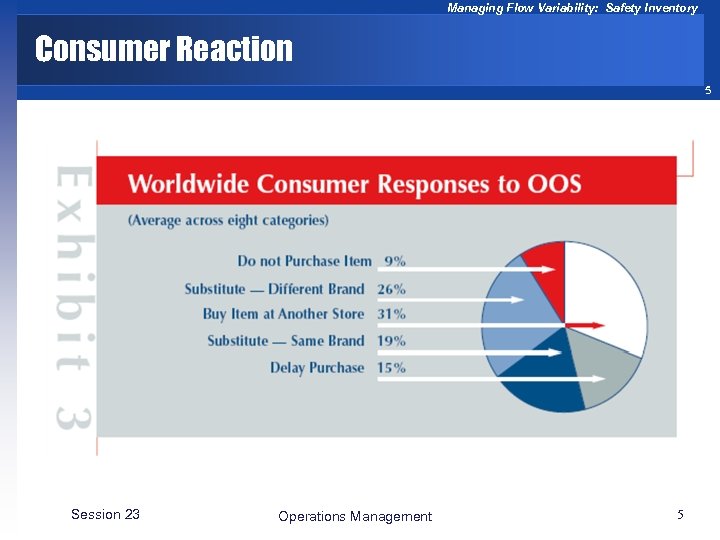
Managing Flow Variability: Safety Inventory Consumer Reaction 5 Session 23 Operations Management 5

Managing Flow Variability: Safety Inventory What can be done to minimize shortages? 6 Better forecast Produce to order and not to stock – Is it always feasible? Have large inventory levels Order the right quantity – What do we mean by the right quantity? Session 23 Operations Management 6

Managing Flow Variability: Safety Inventory Uncertain Demand 7 What is the objective? – Minimize the expected cost (Maximize the expected profits). What are the decision variables? – The optimal purchasing quantity, or the optimal inventory level. Session 23 Operations Management 7

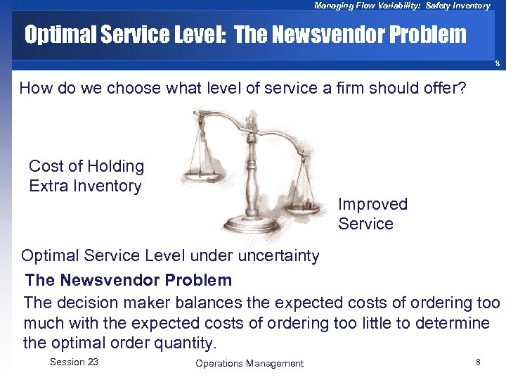
Managing Flow Variability: Safety Inventory Optimal Service Level: The Newsvendor Problem 8 How do we choose what level of service a firm should offer? Cost of Holding Extra Inventory Improved Service Optimal Service Level under uncertainty The Newsvendor Problem The decision maker balances the expected costs of ordering too much with the expected costs of ordering too little to determine the optimal order quantity. Session 23 Operations Management 8

Managing Flow Variability: Safety Inventory News Vendor Model 9 Assumptions – Demand is random – Distribution of demand is known – No initial inventory – Set-up cost is equal to zero – Single period – Zero lead time – Linear costs: • • Session 23 Purchasing (production) Salvage value Revenue Goodwill Operations Management 9

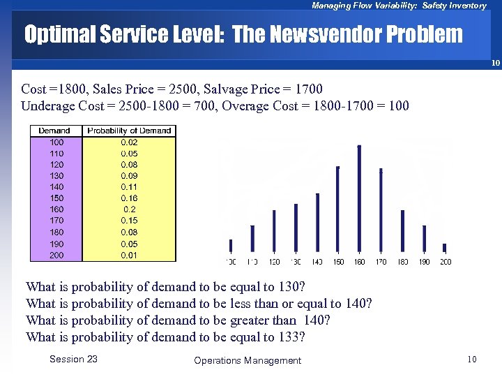
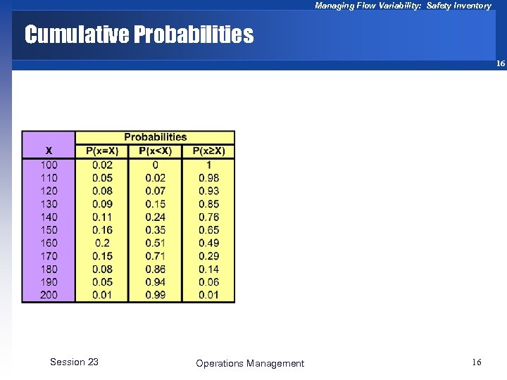
Managing Flow Variability: Safety Inventory Optimal Service Level: The Newsvendor Problem 10 Cost =1800, Sales Price = 2500, Salvage Price = 1700 Underage Cost = 2500 -1800 = 700, Overage Cost = 1800 -1700 = 100 What is probability of demand to be equal to 130? What is probability of demand to be less than or equal to 140? What is probability of demand to be greater than 140? What is probability of demand to be equal to 133? Session 23 Operations Management 10

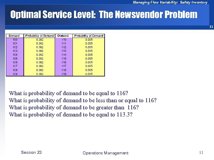
Managing Flow Variability: Safety Inventory Optimal Service Level: The Newsvendor Problem 11 What is probability of demand to be equal to 116? What is probability of demand to be less than or equal to 116? What is probability of demand to be greater than 116? What is probability of demand to be equal to 113. 3? Session 23 Operations Management 11

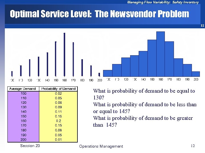
Managing Flow Variability: Safety Inventory Optimal Service Level: The Newsvendor Problem 12 What is probability of demand to be equal to 130? What is probability of demand to be less than or equal to 145? What is probability of demand to be greater than 145? Session 23 Operations Management 12

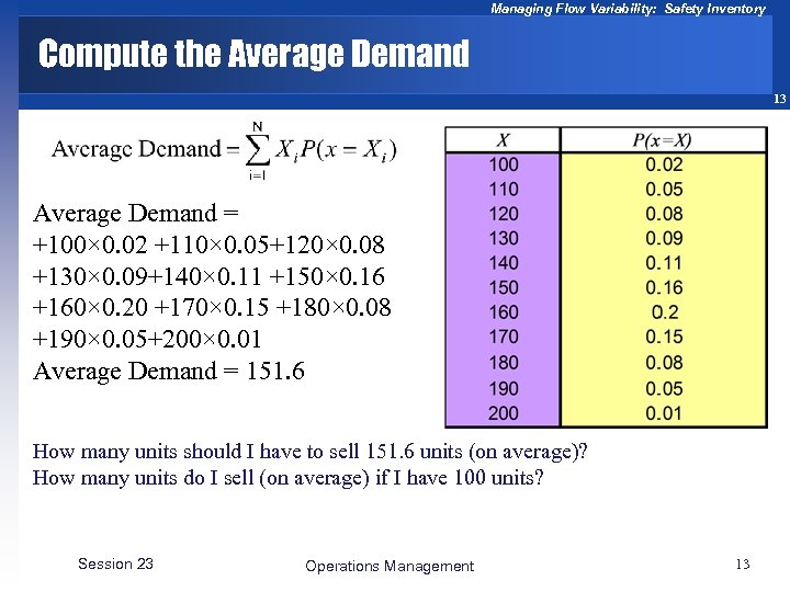
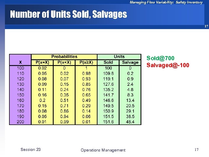
Managing Flow Variability: Safety Inventory Compute the Average Demand 13 Average Demand = +100× 0. 02 +110× 0. 05+120× 0. 08 +130× 0. 09+140× 0. 11 +150× 0. 16 +160× 0. 20 +170× 0. 15 +180× 0. 08 +190× 0. 05+200× 0. 01 Average Demand = 151. 6 How many units should I have to sell 151. 6 units (on average)? How many units do I sell (on average) if I have 100 units? Session 23 Operations Management 13

Managing Flow Variability: Safety Inventory 14 Suppose I have ordered 140 Unities. On average, how many of them are sold? In other words, what is the expected value of the number of sold units? When I can sell all 140 units? I can sell all 140 units if x ≥ 140 Prob(x ≥ 140) = 0. 76 The expected number of units sold –for this part- is (0. 76)(140) = 106. 4 Also, there is 0. 02 probability that I sell 100 units 2 units Also, there is 0. 05 probability that I sell 110 units 5. 5 Also, there is 0. 08 probability that I sell 120 units 9. 6 Also, there is 0. 09 probability that I sell 130 units 11. 7 106. 4 + 2 + 5. 5 + 9. 6 + 11. 7 = 135. 2 Session 23 Operations Management 14

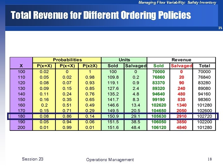
Managing Flow Variability: Safety Inventory 15 Suppose I have ordered 140 Unities. On average, how many of them are salvaged? In other words, what is the expected value of the number of salvaged units? 0. 02 probability that I sell 100 units. In that case 40 units are salvaged 0. 02(40) =. 8 0. 05 probability to sell 110 30 salvaged 0. 05(30)= 1. 5 0. 08 probability to sell 120 20 salvaged 0. 08(20) = 1. 6 0. 09 probability to sell 130 10 salvaged 0. 09(10) =0. 9 0. 8 + 1. 5 + 1. 6 + 0. 9 = 4. 8 Total number Sold 135. 2 @ 700 = 94640 Total number Salvaged 4. 8 @ -100 = -480 Expected Profit = 94640 – 480 = 94, 160 Session 23 Operations Management 15

Managing Flow Variability: Safety Inventory Cumulative Probabilities 16 Session 23 Operations Management 16

Managing Flow Variability: Safety Inventory Number of Units Sold, Salvages 17 Sold@700 Salvaged@-100 Session 23 Operations Management 17

Managing Flow Variability: Safety Inventory Total Revenue for Different Ordering Policies 18 Session 23 Operations Management 18

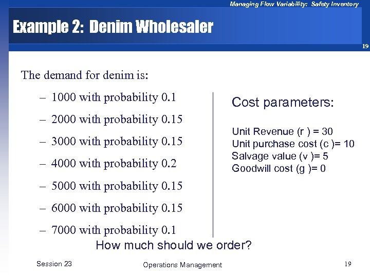
Managing Flow Variability: Safety Inventory Example 2: Denim Wholesaler 19 The demand for denim is: – 1000 with probability 0. 1 – 2000 with probability 0. 15 – 3000 with probability 0. 15 – 4000 with probability 0. 2 Cost parameters: Unit Revenue (r ) = 30 Unit purchase cost (c )= 10 Salvage value (v )= 5 Goodwill cost (g )= 0 – 5000 with probability 0. 15 – 6000 with probability 0. 15 – 7000 with probability 0. 1 How much should we order? Session 23 Operations Management 19

Managing Flow Variability: Safety Inventory 20

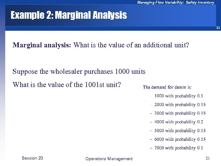
Managing Flow Variability: Safety Inventory Example 2: Marginal Analysis 21 Marginal analysis: What is the value of an additional unit? Suppose the wholesaler purchases 1000 units What is the value of the 1001 st unit? Session 23 Operations Management 21

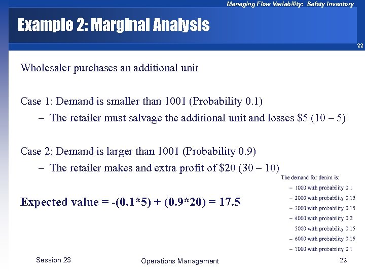
Managing Flow Variability: Safety Inventory Example 2: Marginal Analysis 22 Wholesaler purchases an additional unit Case 1: Demand is smaller than 1001 (Probability 0. 1) – The retailer must salvage the additional unit and losses $5 (10 – 5) Case 2: Demand is larger than 1001 (Probability 0. 9) – The retailer makes and extra profit of $20 (30 – 10) Expected value = -(0. 1*5) + (0. 9*20) = 17. 5 Session 23 Operations Management 22

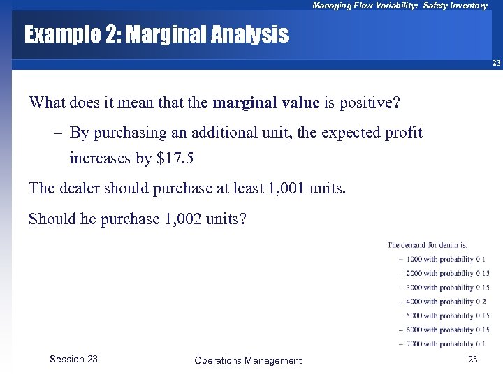
Managing Flow Variability: Safety Inventory Example 2: Marginal Analysis 23 What does it mean that the marginal value is positive? – By purchasing an additional unit, the expected profit increases by $17. 5 The dealer should purchase at least 1, 001 units. Should he purchase 1, 002 units? Session 23 Operations Management 23

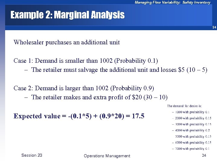
Managing Flow Variability: Safety Inventory Example 2: Marginal Analysis 24 Wholesaler purchases an additional unit Case 1: Demand is smaller than 1002 (Probability 0. 1) – The retailer must salvage the additional unit and losses $5 (10 – 5) Case 2: Demand is larger than 1002 (Probability 0. 9) – The retailer makes and extra profit of $20 (30 – 10) Expected value = -(0. 1*5) + (0. 9*20) = 17. 5 Session 23 Operations Management 24

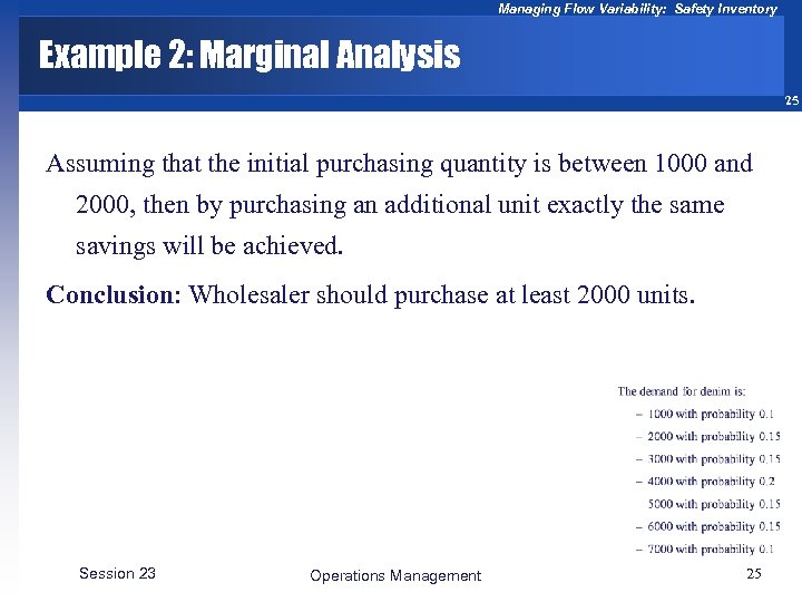
Managing Flow Variability: Safety Inventory Example 2: Marginal Analysis 25 Assuming that the initial purchasing quantity is between 1000 and 2000, then by purchasing an additional unit exactly the same savings will be achieved. Conclusion: Wholesaler should purchase at least 2000 units. Session 23 Operations Management 25

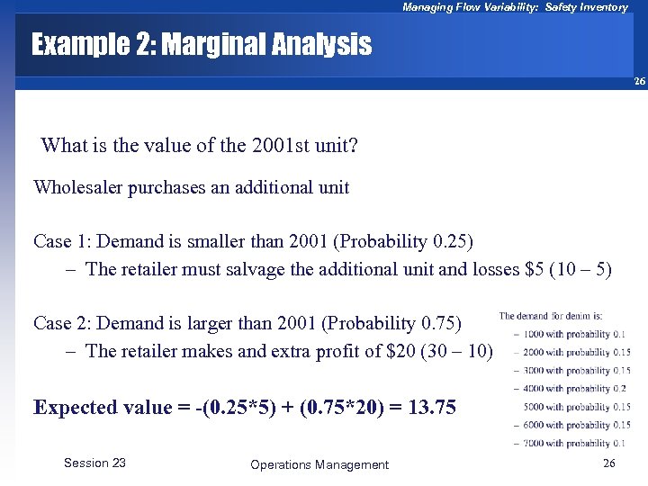
Managing Flow Variability: Safety Inventory Example 2: Marginal Analysis 26 What is the value of the 2001 st unit? Wholesaler purchases an additional unit Case 1: Demand is smaller than 2001 (Probability 0. 25) – The retailer must salvage the additional unit and losses $5 (10 – 5) Case 2: Demand is larger than 2001 (Probability 0. 75) – The retailer makes and extra profit of $20 (30 – 10) Expected value = -(0. 25*5) + (0. 75*20) = 13. 75 Session 23 Operations Management 26

Managing Flow Variability: Safety Inventory Example 2: Marginal Analysis 27 Why does the marginal value of an additional unit decrease, as the purchasing quantity increases? – Expected cost of an additional unit increases – Expected savings of an additional unit decreases Session 23 Operations Management 27

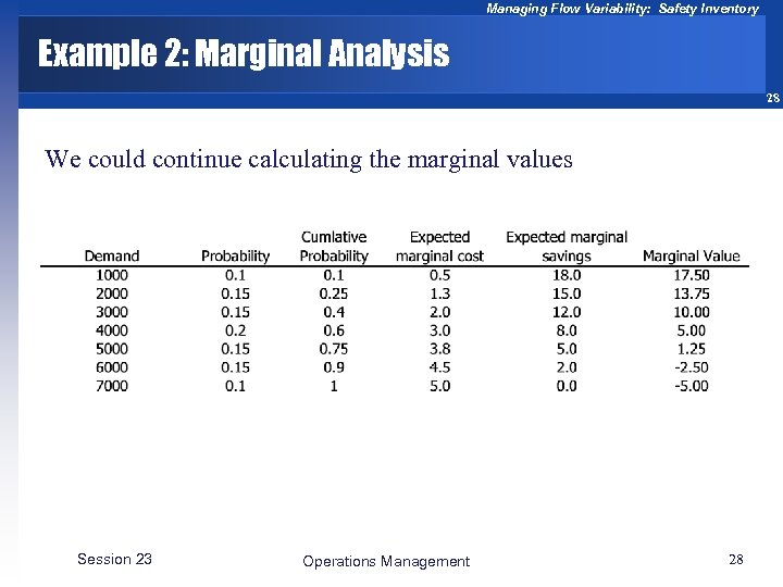
Managing Flow Variability: Safety Inventory Example 2: Marginal Analysis 28 We could continue calculating the marginal values Session 23 Operations Management 28

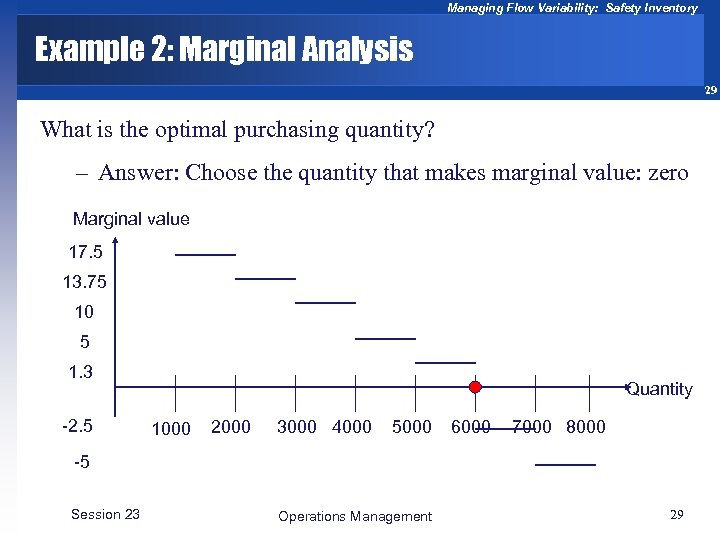
Managing Flow Variability: Safety Inventory Example 2: Marginal Analysis 29 What is the optimal purchasing quantity? – Answer: Choose the quantity that makes marginal value: zero Marginal value 17. 5 13. 75 10 5 1. 3 -2. 5 Quantity 1000 2000 3000 4000 5000 6000 7000 8000 -5 Session 23 Operations Management 29

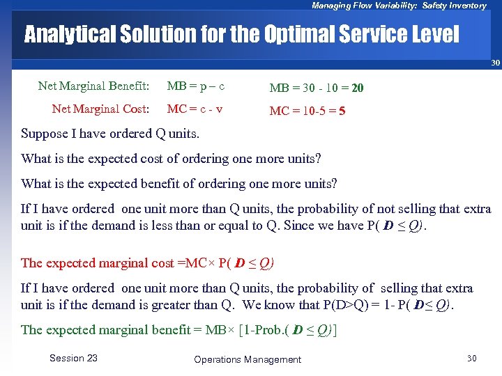
Managing Flow Variability: Safety Inventory Analytical Solution for the Optimal Service Level 30 Net Marginal Benefit: MB = p – c MB = 30 - 10 = 20 Net Marginal Cost: MC = c - v MC = 10 -5 = 5 Suppose I have ordered Q units. What is the expected cost of ordering one more units? What is the expected benefit of ordering one more units? If I have ordered one unit more than Q units, the probability of not selling that extra unit is if the demand is less than or equal to Q. Since we have P( D ≤ Q). The expected marginal cost =MC× P( D ≤ Q) If I have ordered one unit more than Q units, the probability of selling that extra unit is if the demand is greater than Q. We know that P(D>Q) = 1 - P( D≤ Q). The expected marginal benefit = MB× [1 -Prob. ( D ≤ Q)] Session 23 Operations Management 30

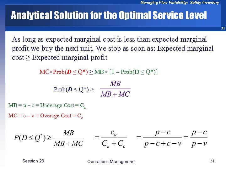
Managing Flow Variability: Safety Inventory Analytical Solution for the Optimal Service Level 31 As long as expected marginal cost is less than expected marginal profit we buy the next unit. We stop as soon as: Expected marginal cost ≥ Expected marginal profit MC×Prob(D ≤ Q*) ≥ MB× [1 – Prob(D ≤ Q*)] Prob(D ≤ Q*) ≥ MB = p – c = Underage Cost = Cu MC = c – v = Overage Cost = Co Session 23 Operations Management 31

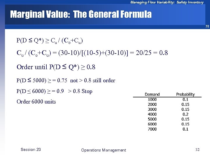
Managing Flow Variability: Safety Inventory Marginal Value: The General Formula 32 P(D ≤ Q*) ≥ Cu / (Co+Cu) = (30 -10)/[(10 -5)+(30 -10)] = 20/25 = 0. 8 Order until P(D ≤ Q*) ≥ 0. 8 P(D ≤ 5000) ≥ = 0. 75 not > 0. 8 still order P(D ≤ 6000) ≥ = 0. 9 > 0. 8 Stop Order 6000 units Session 23 Operations Management 32

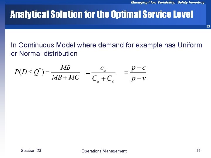
Managing Flow Variability: Safety Inventory Analytical Solution for the Optimal Service Level 33 In Continuous Model where demand for example has Uniform or Normal distribution Session 23 Operations Management 33

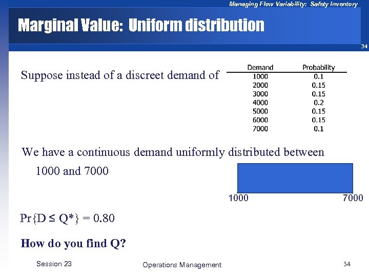
Managing Flow Variability: Safety Inventory Marginal Value: Uniform distribution 34 Suppose instead of a discreet demand of We have a continuous demand uniformly distributed between 1000 and 7000 1000 7000 Pr{D ≤ Q*} = 0. 80 How do you find Q? Session 23 Operations Management 34

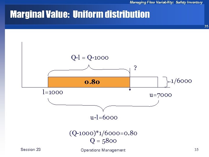
Managing Flow Variability: Safety Inventory Marginal Value: Uniform distribution 35 Q-l = Q-1000 ? 0. 80 l=1000 1/6000 u=7000 u-l=6000 (Q-1000)*1/6000=0. 80 Q = 5800 Session 23 Operations Management 35

Managing Flow Variability: Safety Inventory Type-1 Service Level 36 What is the meaning of the number 0. 80? F(Q) = (30 – 10) / (30 – 5) = 0. 8 – Pr {demand is smaller than Q} = – Pr {No shortage} = – Pr {All the demand is satisfied from stock} = 0. 80 It is optimal to ensure that 80% of the time all the demand is satisfied. Session 23 Operations Management 36

Managing Flow Variability: Safety Inventory Marginal Value: Normal Distribution 37 Suppose the demand is normally distributed with a mean of 4000 and a standard deviation of 1000. What is the optimal order quantity? Notice: F(Q) = 0. 80 is correct for all distributions. We only need to find the right value of Q assuming the normal distribution. Session 23 Operations Management 37

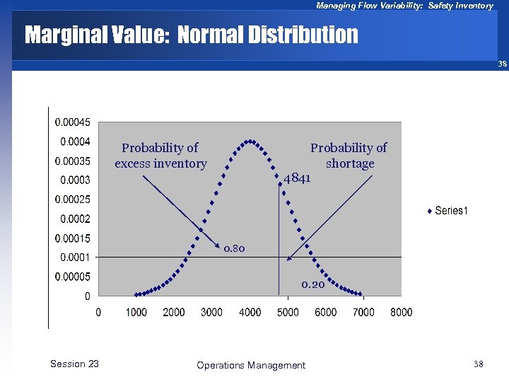
Managing Flow Variability: Safety Inventory Marginal Value: Normal Distribution 38 Probability of excess inventory Probability of shortage 4841 0. 80 0. 20 Session 23 Operations Management 38

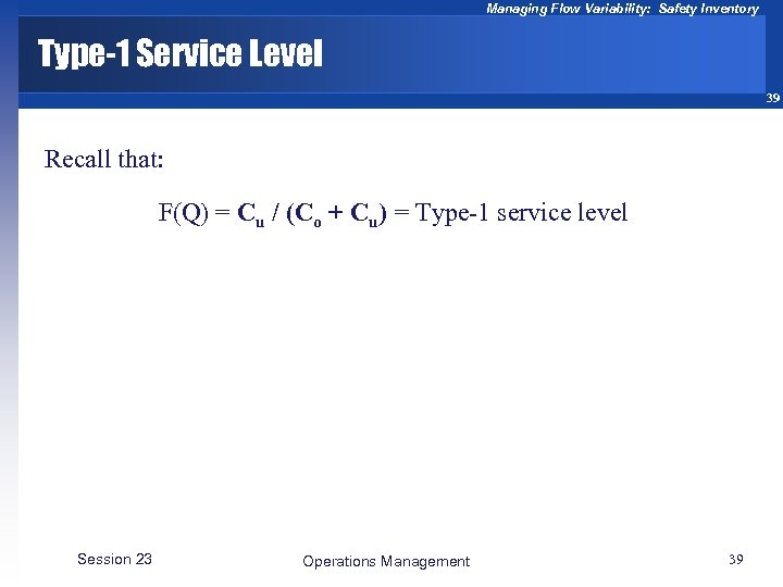
Managing Flow Variability: Safety Inventory Type-1 Service Level 39 Recall that: F(Q) = Cu / (Co + Cu) = Type-1 service level Session 23 Operations Management 39

Managing Flow Variability: Safety Inventory Type-1 Service Level 40 Is it correct to set the service level to 0. 8? Shouldn’t we aim to provide 100% serviceability? Session 23 Operations Management 40

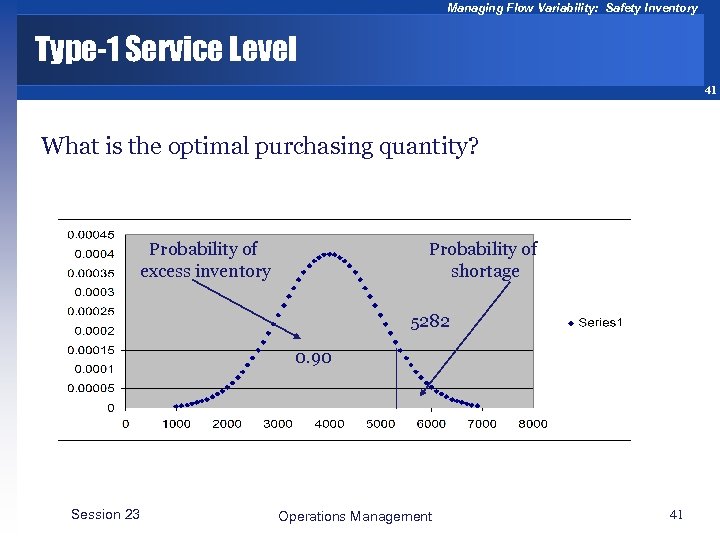
Managing Flow Variability: Safety Inventory Type-1 Service Level 41 What is the optimal purchasing quantity? Probability of excess inventory Probability of shortage 5282 0. 90 Session 23 Operations Management 41

Managing Flow Variability: Safety Inventory Type-1 Service Level 42 How do you determine the service level? For normal distribution, it is always optimal to have: Mean + z*Standard deviation µ + zs The service level determines the value of Z zs is the level of safety stock m +zs is the base stock (order-up-to level) Session 23 Operations Management 42

Managing Flow Variability: Safety Inventory Type-1 Service Level 43 Given a service level, how do we calculate z? From our normal table or From Excel – Normsinv(service level) Session 23 Operations Management 43

Managing Flow Variability: Safety Inventory Additional Example 44 Your store is selling calendars, which cost you $6. 00 and sell for $12. 00 You cannot predict demand for the calendars with certainty. Data from previous years suggest that demand is well described by a normal distribution with mean value 60 and standard deviation 10. Calendars which remain unsold after January are returned to the publisher for a $2. 00 "salvage" credit. There is only one opportunity to order the calendars. What is the right number of calendars to order? Session 23 Operations Management 44

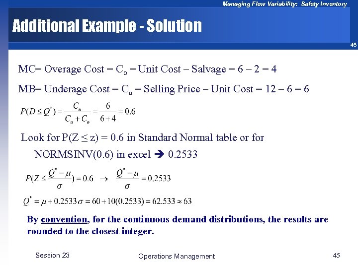
Managing Flow Variability: Safety Inventory Additional Example - Solution 45 MC= Overage Cost = Co = Unit Cost – Salvage = 6 – 2 = 4 MB= Underage Cost = Cu = Selling Price – Unit Cost = 12 – 6 = 6 Look for P(Z ≤ z) = 0. 6 in Standard Normal table or for NORMSINV(0. 6) in excel 0. 2533 By convention, for the continuous demand distributions, the results are rounded to the closest integer. Session 23 Operations Management 45

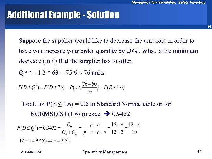
Managing Flow Variability: Safety Inventory Additional Example - Solution 46 Suppose the supplier would like to decrease the unit cost in order to have you increase your order quantity by 20%. What is the minimum decrease (in $) that the supplier has to offer. Qnew = 1. 2 * 63 = 75. 6 ~ 76 units Look for P(Z ≤ 1. 6) = 0. 6 in Standard Normal table or for NORMSDIST(1. 6) in excel 0. 9452 Session 23 Operations Management 46

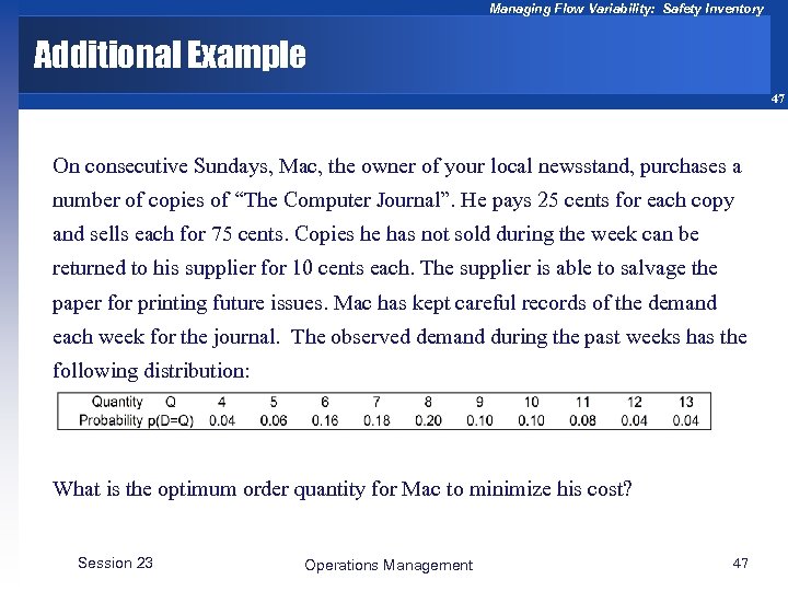
Managing Flow Variability: Safety Inventory Additional Example 47 On consecutive Sundays, Mac, the owner of your local newsstand, purchases a number of copies of “The Computer Journal”. He pays 25 cents for each copy and sells each for 75 cents. Copies he has not sold during the week can be returned to his supplier for 10 cents each. The supplier is able to salvage the paper for printing future issues. Mac has kept careful records of the demand each week for the journal. The observed demand during the past weeks has the following distribution: What is the optimum order quantity for Mac to minimize his cost? Session 23 Operations Management 47

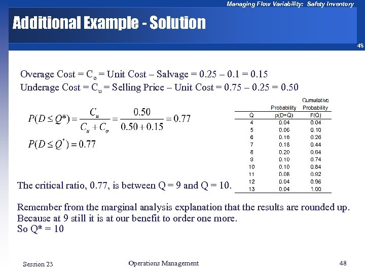
Managing Flow Variability: Safety Inventory Additional Example - Solution 48 Overage Cost = Co = Unit Cost – Salvage = 0. 25 – 0. 1 = 0. 15 Underage Cost = Cu = Selling Price – Unit Cost = 0. 75 – 0. 25 = 0. 50 The critical ratio, 0. 77, is between Q = 9 and Q = 10. Remember from the marginal analysis explanation that the results are rounded up. Because at 9 still it is at our benefit to order one more. So Q* = 10 Session 23 Operations Management 48