Managing Facilitating Goods Replenishment order Factory Production Delay

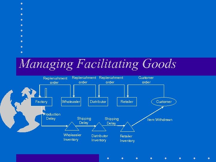Managing Facilitating Goods Replenishment order Factory Production Delay Replenishment order Wholesaler Distributor Shipping Delay Wholesaler Inventory Retailer Shipping Delay Distributor Inventory Customer order Customer Item Withdrawn Retailer Inventory

Learning Objectives • Discuss the role of information technology in managing inventories. • Describe the functions and costs of an inventory system. • Determine the order quantity. • Determine the reorder point and safety stock for inventory systems with uncertain demand. • Design a continuous or periodic review inventory-control system. • Conduct an ABC analysis of inventory items. • Determine the order quantity for the single-period inventory case. • Describe the rationale behind the retail discounting model.

Role of Inventory in Services • • • Decoupling inventories Seasonal inventories Speculative inventories Cyclical inventories In-transit inventories Safety stocks

Considerations in Inventory Systems • Type of customer demand • Planning time horizon • Replenishment lead time • Constraints and relevant costs

Relevant Inventory Costs • Ordering costs • Receiving and inspections costs • Holding or carrying costs • Shortage costs

Inventory Management Questions • What should be the order quantity (Q)? • When should an order be placed, called a reorder point (ROP)? • How much safety stock (SS) should be maintained?

Inventory Models • Economic Order Quantity (EOQ) • Special Inventory Models With Quantity Discounts Planned Shortages • Demand Uncertainty - Safety Stocks • Inventory Control Systems Continuous-Review (Q, r) Periodic-Review (order-up-to) • Single Period Inventory Model

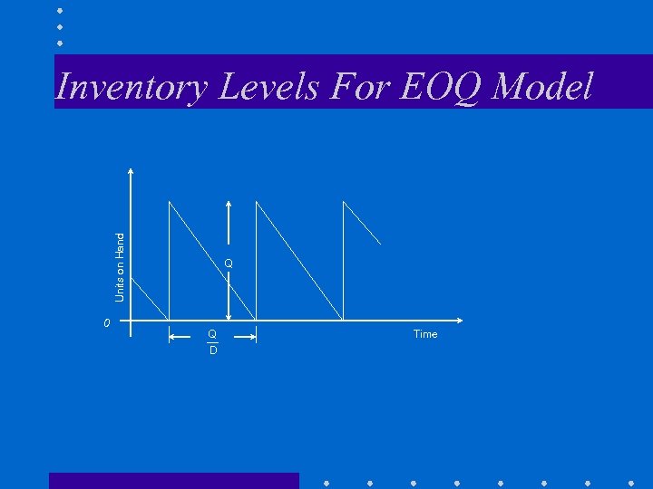Units on Hand Inventory Levels For EOQ Model 0 Q Q D Time

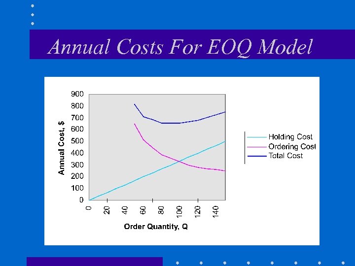Annual Costs For EOQ Model

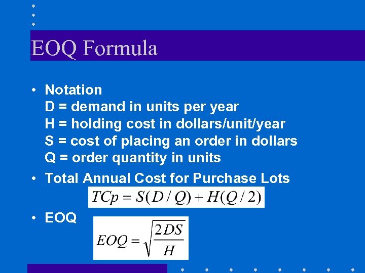EOQ Formula • Notation D = demand in units per year H = holding cost in dollars/unit/year S = cost of placing an order in dollars Q = order quantity in units • Total Annual Cost for Purchase Lots • EOQ

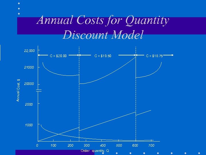Annual Costs for Quantity Discount Model 22, 000 C = $20. 00 C = $19. 50 C = $18. 75 Annual Cost, $ 21000 2000 1000 0 100 200 300 400 Order quantity, Q 500 600 700

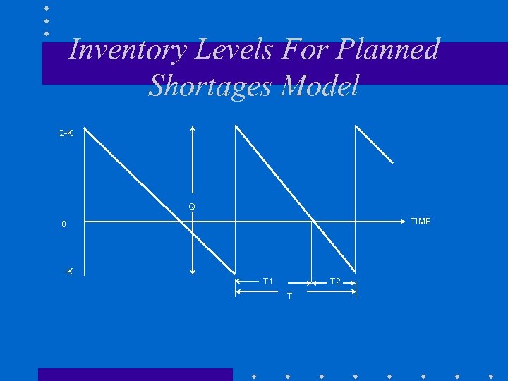Inventory Levels For Planned Shortages Model Q-K Q TIME 0 -K T 1 T 2 T

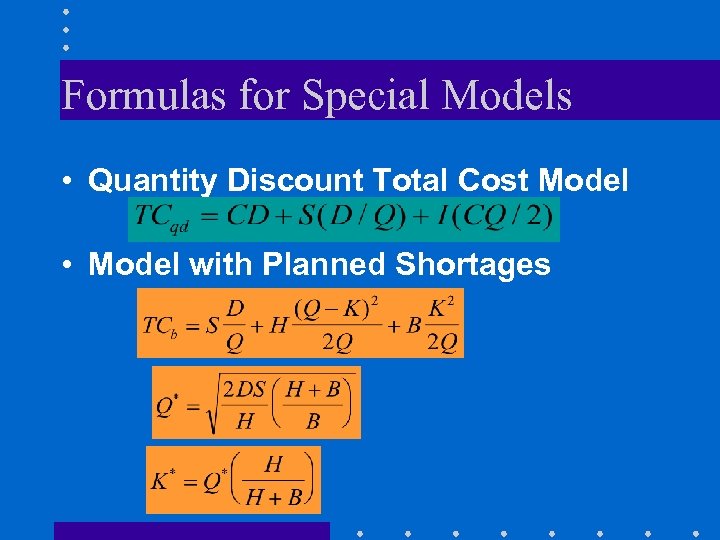Formulas for Special Models • Quantity Discount Total Cost Model • Model with Planned Shortages

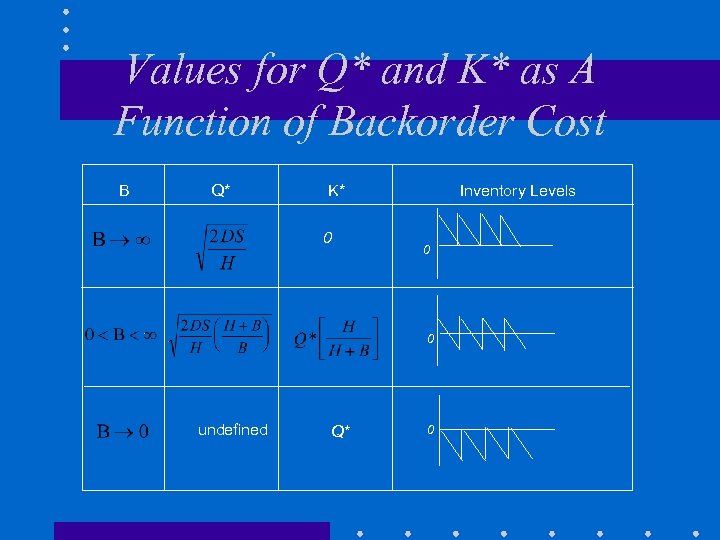Values for Q* and K* as A Function of Backorder Cost B Q* K* 0 Inventory Levels 0 0 undefined Q* 0

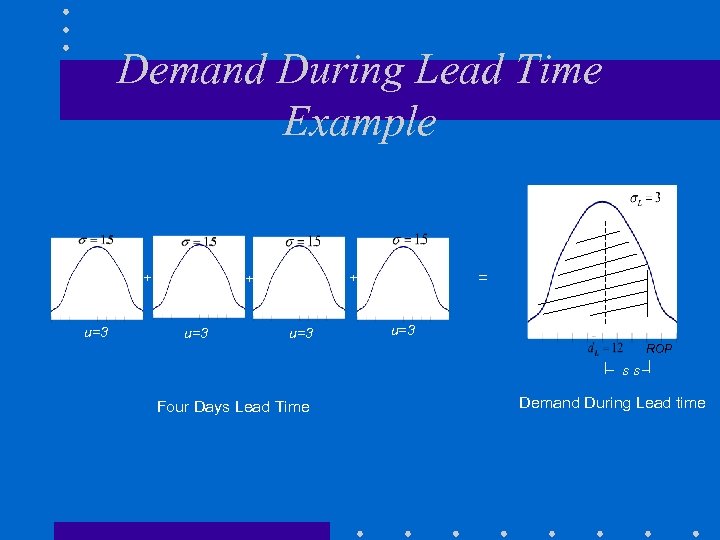Demand During Lead Time Example + u=3 = + + u=3 ROP ss Four Days Lead Time Demand During Lead time

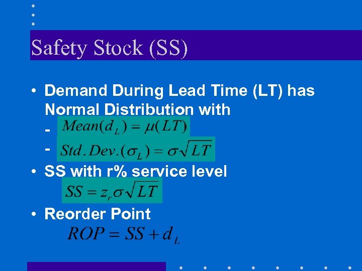Safety Stock (SS) • Demand During Lead Time (LT) has Normal Distribution with • SS with r% service level • Reorder Point

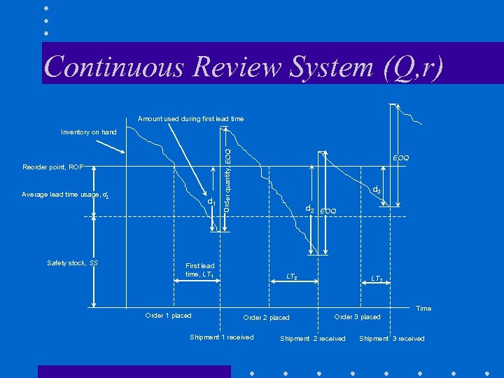Continuous Review System (Q, r) Amount used during first lead time Reorder point, ROP Average lead time usage, d. L Safety stock, SS d 1 Order quantity, EOQ Inventory on hand EOQ d 3 d 2 EOQ First lead time, LT 1 Order 1 placed LT 2 LT 3 Time Order 2 placed Shipment 1 received Order 3 placed Shipment 2 received Shipment 3 received

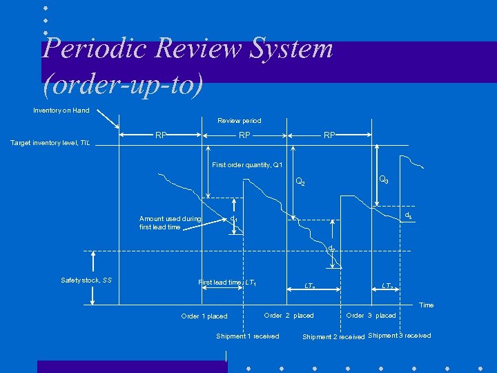Periodic Review System (order-up-to) Inventory on Hand Review period Target inventory level, TIL RP RP RP First order quantity, Q 1 Q 3 Q 2 d 3 d 1 Amount used during first lead time d 2 Safety stock, SS First lead time, LT 1 LT 2 LT 3 Time Order 1 placed Order 2 placed Shipment 1 received Order 3 placed Shipment 2 received Shipment 3 received

Inventory Control Systems • Continuous Review System • Periodic Review System

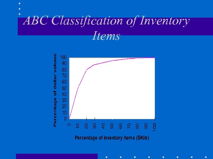ABC Classification of Inventory Items A B C

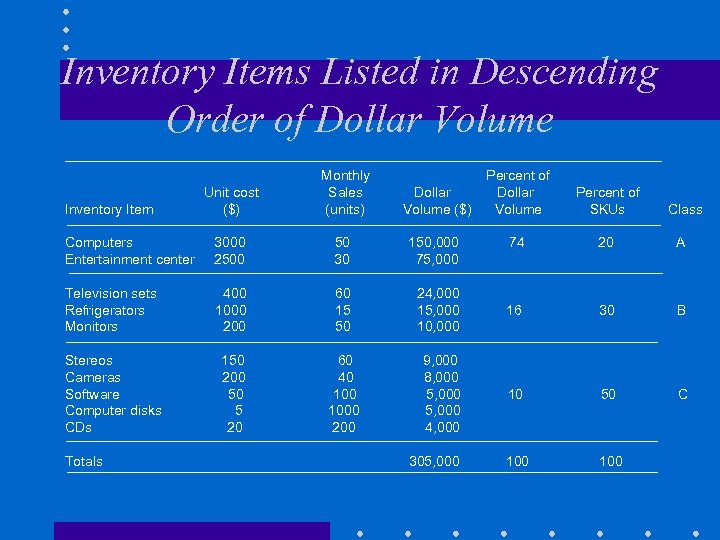Inventory Items Listed in Descending Order of Dollar Volume Unit cost ($) Monthly Sales (units) Dollar Volume ($) Computers Entertainment center 3000 2500 50 30 150, 000 75, 000 Television sets Refrigerators Monitors 400 1000 200 60 15 50 Stereos Cameras Software Computer disks CDs 150 200 50 5 20 60 40 1000 200 Inventory Item Totals Percent of Dollar Volume Percent of SKUs 74 20 A 24, 000 15, 000 10, 000 16 30 B 9, 000 8, 000 5, 000 4, 000 10 50 C 100 305, 000 Class

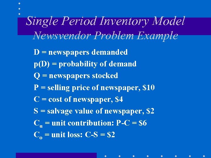Single Period Inventory Model Newsvendor Problem Example D = newspapers demanded p(D) = probability of demand Q = newspapers stocked P = selling price of newspaper, $10 C = cost of newspaper, $4 S = salvage value of newspaper, $2 Cu = unit contribution: P-C = $6 Co = unit loss: C-S = $2

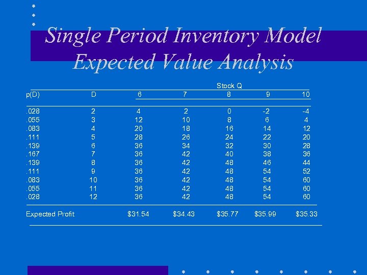Single Period Inventory Model Expected Value Analysis p(D) D 6 7 Stock Q 8 . 028. 055. 083. 111. 139. 167. 139. 111. 083. 055. 028 2 3 4 5 6 7 8 9 10 11 12 4 12 20 28 36 36 2 10 18 26 34 42 42 42 0 8 16 24 32 40 48 48 48 -2 6 14 22 30 38 46 54 54 -4 4 12 20 28 36 44 52 60 60 60 $31. 54 $34. 43 $35. 77 $35. 99 $35. 33 Expected Profit 9 10

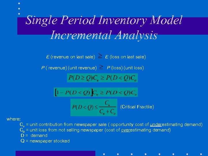Single Period Inventory Model Incremental Analysis E (revenue on last sale) P ( revenue) (unit revenue) E (loss on last sale) P (loss) (unit loss) (Critical Fractile) where: Cu = unit contribution from newspaper sale ( opportunity cost of underestimating demand) Co = unit loss from not selling newspaper (cost of overestimating demand) D = demand Q = newspaper stocked

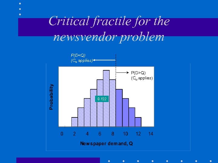Critical fractile for the newsvendor problem P(DQ) (Cu applies) 0. 722

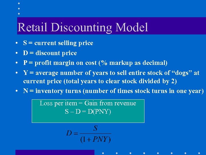Retail Discounting Model • • S = current selling price D = discount price P = profit margin on cost (% markup as decimal) Y = average number of years to sell entire stock of “dogs” at current price (total years to clear stock divided by 2) • N = inventory turns (number of times stock turns in one year) Loss per item = Gain from revenue S – D = D(PNY)

Topics for Discussion • Discuss the functions of inventory for different organizations in the supply chain. • How would one find values for inventory costs? • How can information technology create a competitive advantage through inventory management? • How valid are the assumptions for the EOQ model? • How is a service level determined for inventory items? • What inventory model would apply to service capacity such as seats on an aircraft?

Interactive Exercise The class engages in an estimation of the cost of a 12 -ounce serving of Coke in various situations (e. g. , supermarket, convenience store, fast-food restaurant, sit-down restaurant, and ballpark). What explains the differences?