Managerial Economics Chapter Two.pptx
- Количество слайдов: 50

Managerial Economics & Business Strategy Chapter 2 Market Forces: Demand Supply Mc. Graw-Hill/Irwin Michael R. Baye, Managerial Economics and Business Strategy Copyright © 2008 by the Mc. Graw-Hill Companies, Inc. All rights reserved.
2 -2 Overview I. Market Demand Curve – The Demand Function – Determinants of Demand – Consumer Surplus II. Market Supply Curve – The Supply Function – Supply Shifters – Producer Surplus III. Market Equilibrium IV. Price Restrictions V. Comparative Statics

+ The Demand Schedule for Jeans in a Small Foreign Market
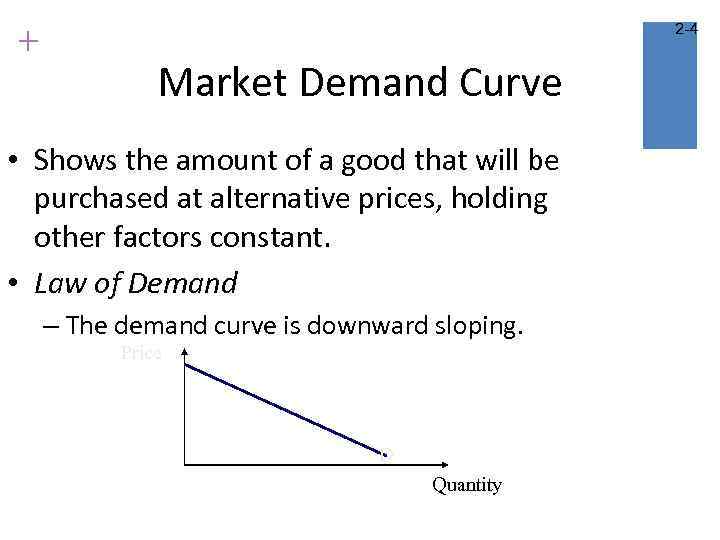
+ 2 -4 Market Demand Curve • Shows the amount of a good that will be purchased at alternative prices, holding other factors constant. • Law of Demand – The demand curve is downward sloping. Price D Quantity

+ Changes in Demand D 1 – normal good D 2 – inferior good
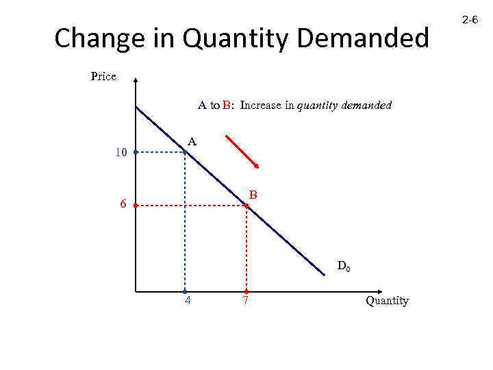
Change in Quantity Demanded Price A to B: Increase in quantity demanded 10 A B 6 D 0 4 7 Quantity 2 -6
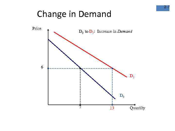
2 -7 Change in Demand Price D 0 to D 1: Increase in Demand 6 D 1 D 0 7 13 Quantity
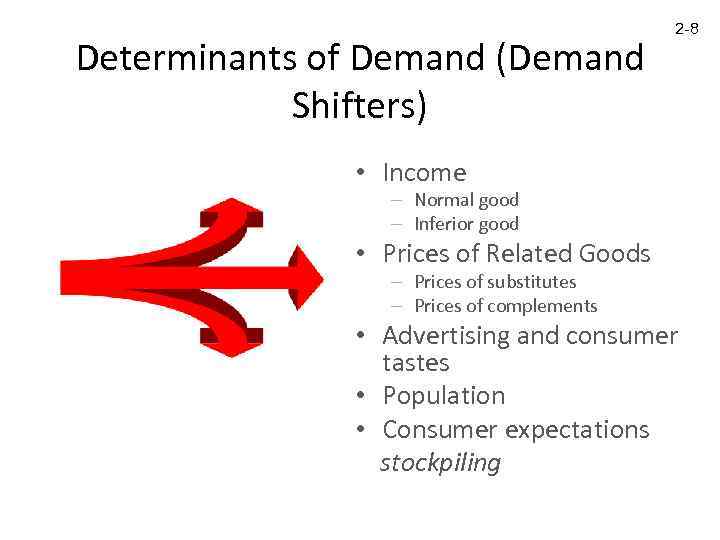
Determinants of Demand (Demand Shifters) 2 -8 • Income – Normal good – Inferior good • Prices of Related Goods – Prices of substitutes – Prices of complements • Advertising and consumer tastes • Population • Consumer expectations stockpiling
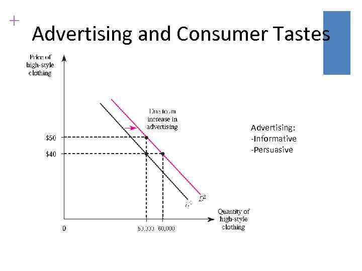
+ Advertising and Consumer Tastes Advertising: -Informative -Persuasive
+ 2 -10 The Demand Function • A general equation representing the demand curve Qxd = f(Px , PY , M, H, ) – Qxd = quantity demand of good X. – Px = price of good X. – PY = price of a related good Y. • Substitute good. • Complement good. – M = income. • Normal good. • Inferior good. – H = any other variable affecting demand Demand function is linear if Qxd is a linear function of all variables.

+ Demand function is linear if Qxd is a linear function of all variables. • Example of a linear demand function:
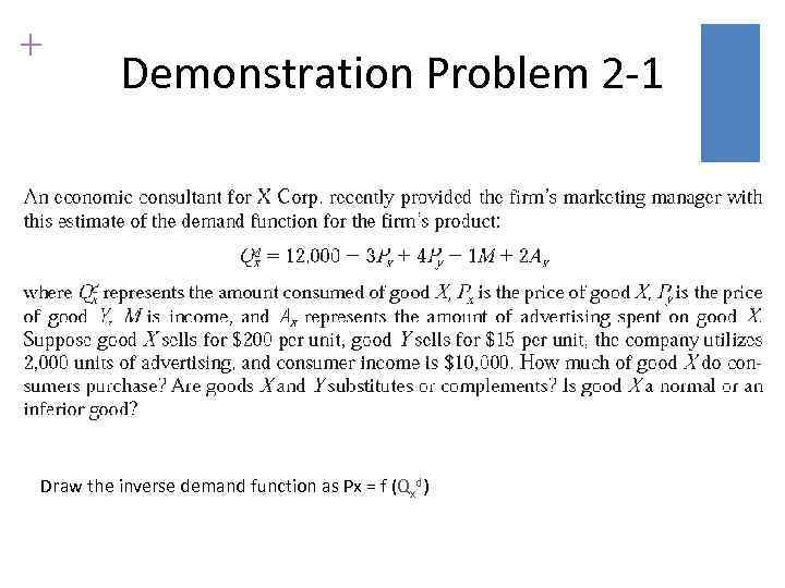
+ Demonstration Problem 2 -1 Draw the inverse demand function as Px = f (Qxd)
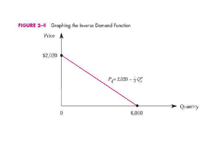
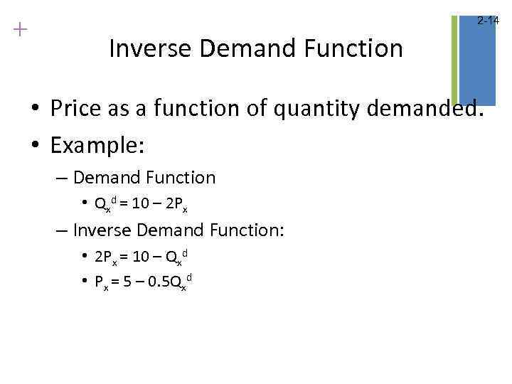
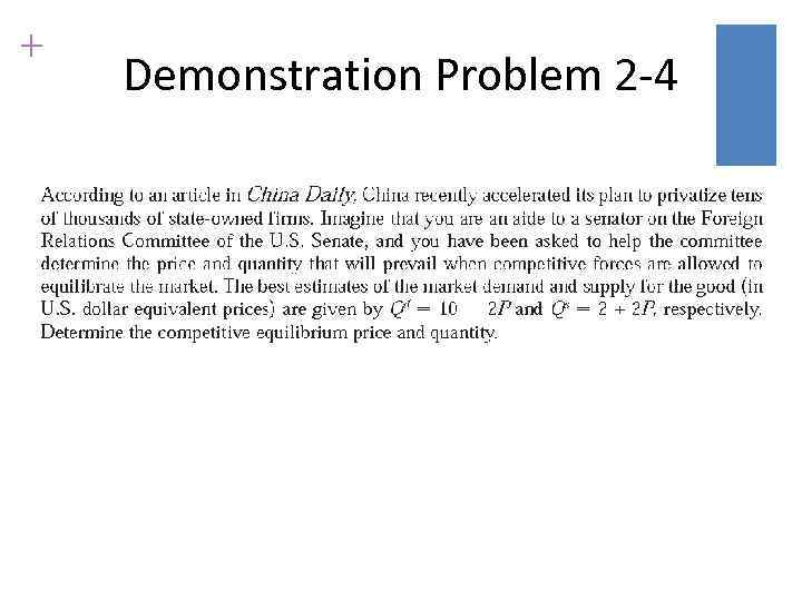
+ 2 -14 Inverse Demand Function • Price as a function of quantity demanded. • Example: – Demand Function • Qxd = 10 – 2 Px – Inverse Demand Function: • 2 Px = 10 – Qxd • Px = 5 – 0. 5 Qxd

2 -15 Consumer Surplus: • The value consumers get from a good but do not have to pay for. • Consumer surplus will prove particularly useful in marketing and other disciplines emphasizing strategies like value pricing and price discrimination.

2 -16 I got a great deal! • That company offers a lot of bang for the buck! • Dell provides good value. • Total value greatly exceeds total amount paid. • Consumer surplus is large.

2 -17 I got a lousy deal! • That car dealer drives a hard bargain! • I almost decided not to buy it! • They tried to squeeze the very last cent from me! • Total amount paid is close to total value. • Consumer surplus is low.

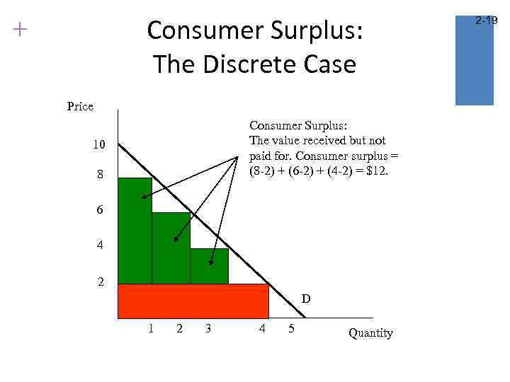
Consumer Surplus: The Discrete Case + Price Consumer Surplus: The value received but not paid for. Consumer surplus = (8 -2) + (6 -2) + (4 -2) = $12. 10 8 6 4 2 D 1 2 3 4 5 Quantity 2 -19
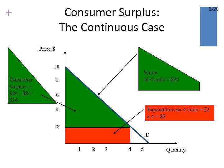
Consumer Surplus: The Continuous Case + 2 -20 Price $ 10 Consumer 8 Surplus = $24 - $8 = $16 Value of 4 units = $24 6 4 Expenditure on 4 units = $2 x 4 = $8 2 D 1 2 3 4 5 Quantity
+ Demonstration Problem 2 -2
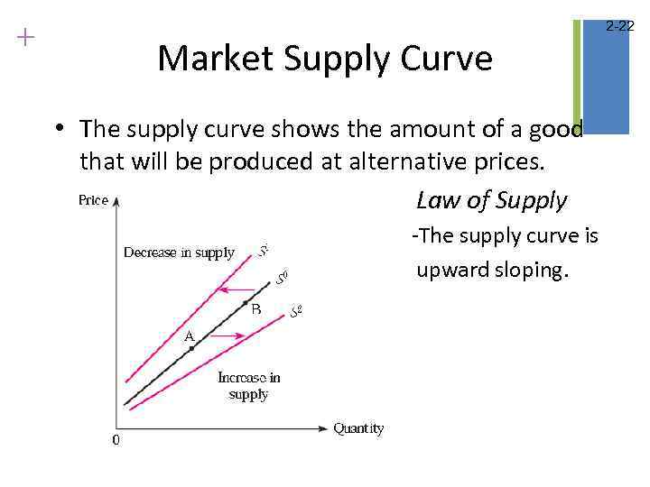
+ Market Supply Curve • The supply curve shows the amount of a good that will be produced at alternative prices. Law of Supply -The supply curve is upward sloping. 2 -22
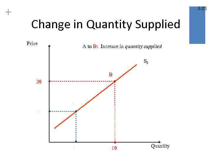
+ 2 -23 Change in Quantity Supplied Price A to B: Increase in quantity supplied S 0 B 20 A 10 5 10 Quantity
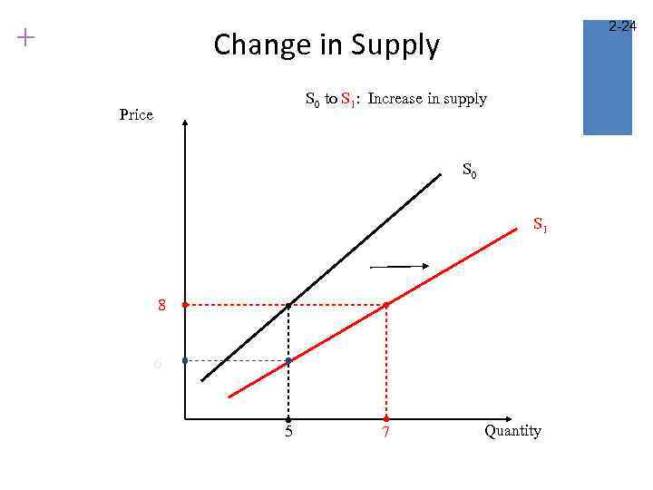
+ 2 -24 Change in Supply S 0 to S 1: Increase in supply Price S 0 S 1 8 6 5 7 Quantity
2 -25 Supply Shifters • Input prices • Technology or government regulations • Number of firms – Entry – Exit • Substitutes in production • Taxes – Excise tax – Ad valorem tax • Producer expectations
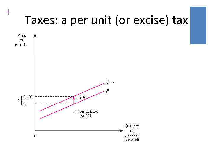
+ Taxes: a per unit (or excise) tax
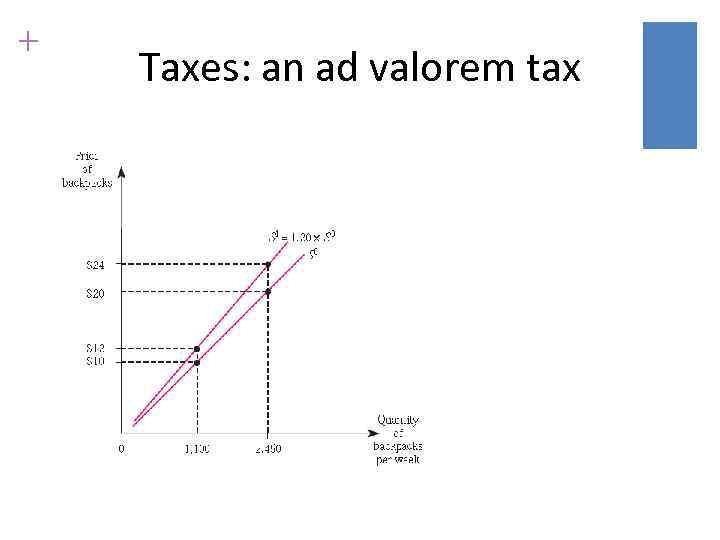
+ Taxes: an ad valorem tax
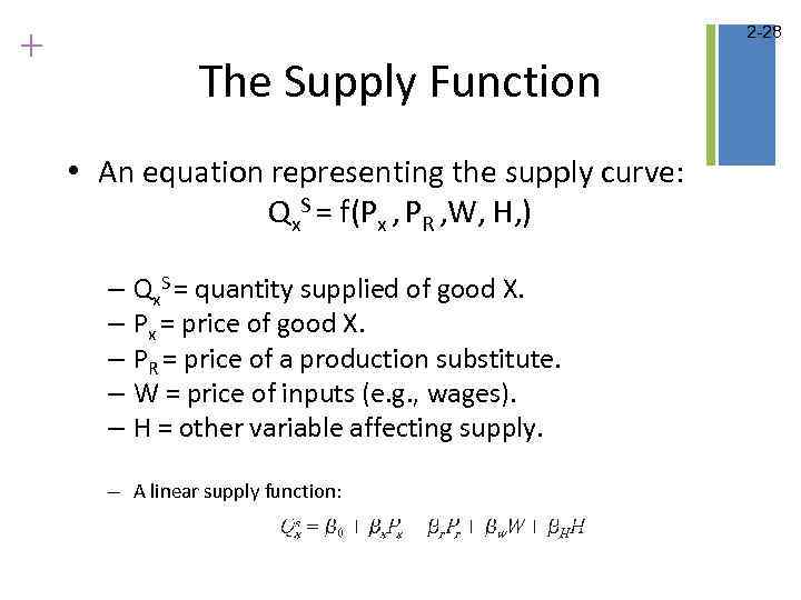
+ 2 -28 The Supply Function • An equation representing the supply curve: Qx. S = f(Px , PR , W, H, ) – Qx. S = quantity supplied of good X. – Px = price of good X. – PR = price of a production substitute. – W = price of inputs (e. g. , wages). – H = other variable affecting supply. – A linear supply function:
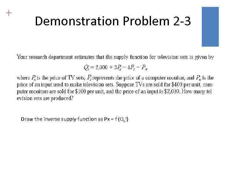
+ Demonstration Problem 2 -3 Draw the inverse supply function as Px = f (Qxs)

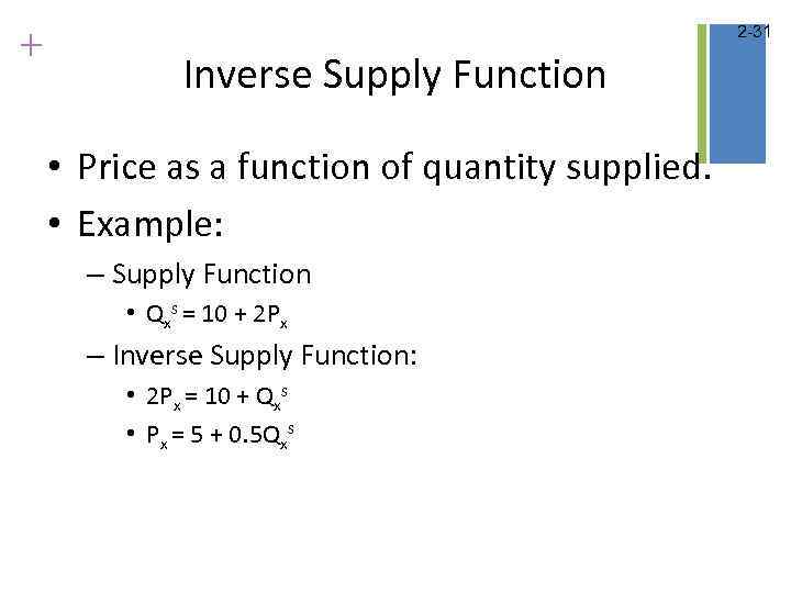
+ 2 -31 Inverse Supply Function • Price as a function of quantity supplied. • Example: – Supply Function • Qxs = 10 + 2 Px – Inverse Supply Function: • 2 Px = 10 + Qxs • Px = 5 + 0. 5 Qxs
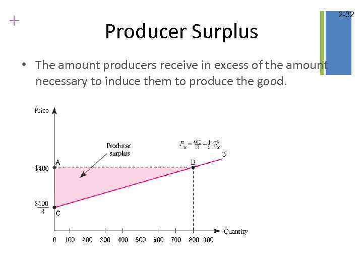
+ Producer Surplus • The amount producers receive in excess of the amount necessary to induce them to produce the good. 2 -32
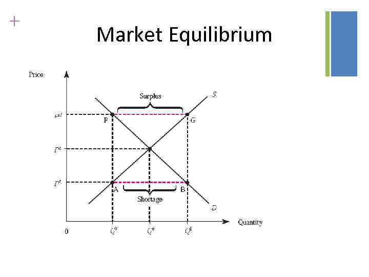
2 -33 Market Equilibrium • The Price (P) that Balances supply and demand – Qx S = Qx d – No shortage or surplus • Steady-state
+ Market Equilibrium
+ Demonstration Problem 2 -4
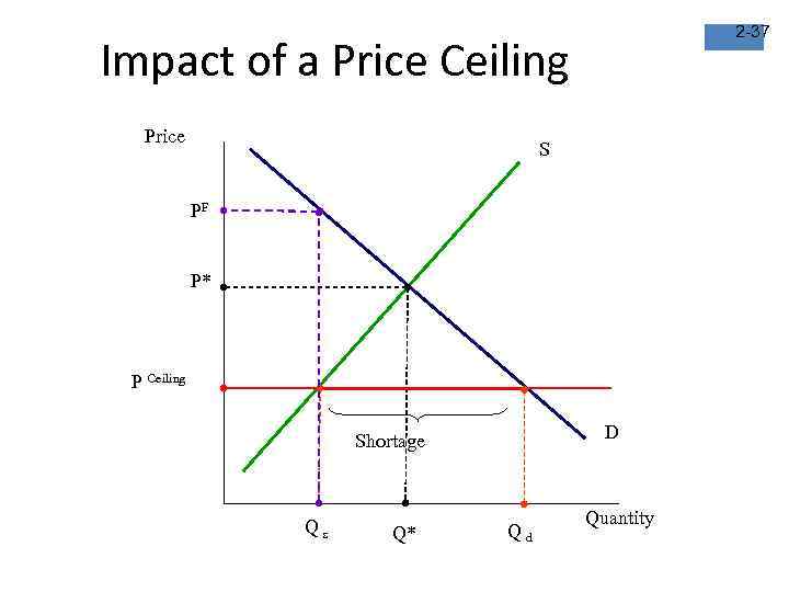
+ Price Restrictions • Price Ceilings – The maximum legal price that can be charged. – Examples: • Prices for important medicaments, basic food items • Price Floors – The minimum legal price that can be charged. – Examples: • Minimum wage. • Agricultural price supports. 2 -36
2 -37 Impact of a Price Ceiling Price S PF P* P Ceiling D Shortage Qs Q* Qd Quantity
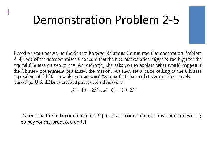
+ Demonstration Problem 2 -5 Determine the full economic price Pf (i. e. the maximum price consumers are willing to pay for the produced units)
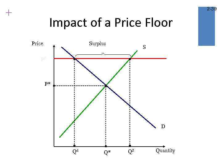
2 -39 + Impact of a Price Floor Price Surplus S PF P* D Qd Q* QS Quantity
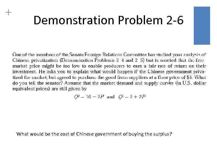
+ Demonstration Problem 2 -6 What would be the cost of Chinese government of buying the surplus?

+ 2 -41 Comparative Static Analysis • How do the equilibrium price and quantity change when a determinant of supply and/or demand change? Note: throughout this analysis we assume no legal restraints such as price floors or ceilings
+ Applications of Demand Supply Analysis • Event: The WSJ reports that the prices of PC components are expected to fall by 5 -8 percent over the next six months. • Scenario 1: You manage a small firm that manufactures PCs. • Scenario 2: You manage a small software company. 2 -42

+ Use Comparative Static Analysis to see the Big Picture! • Comparative static analysis shows how the equilibrium price and quantity will change when a determinant of supply or demand changes. 2 -43
+ 2 -44 Scenario 1: Implications for a Small PC Maker • Step 1: Look for the “Big Picture. ” • Step 2: Organize an action plan (worry about details).
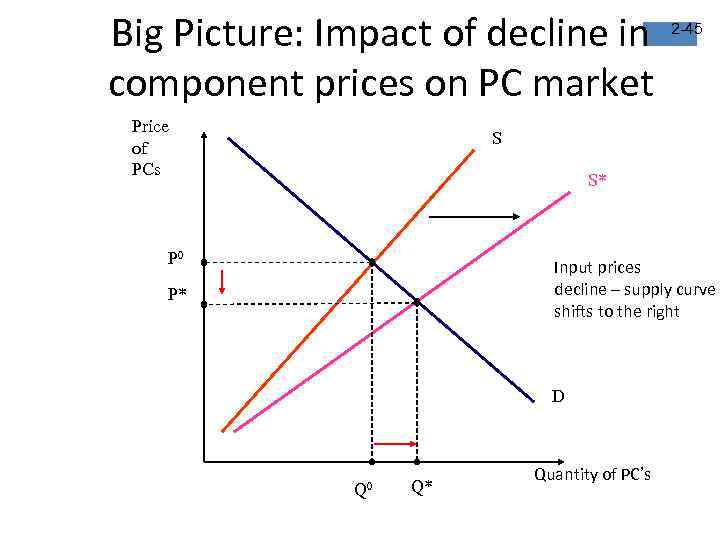
Big Picture: Impact of decline in component prices on PC market Price of PCs 2 -45 S S* P 0 Input prices decline – supply curve shifts to the right P* D Q 0 Q* Quantity of PC’s
+ 2 -46 Big Picture Analysis: PC Market • Equilibrium price of PCs will fall, and equilibrium quantity of computers sold will increase. • Use this to organize an action plan – contracts/suppliers? – inventories? – human resources? – marketing? – do I need quantitative estimates?
+ Scenario 2: Software Maker • More complicated chain of reasoning to arrive at the “Big Picture. ” • Step 1: Use analysis like that in Scenario 1 to deduce that lower component prices will lead to – a lower equilibrium price for computers. – a greater number of computers sold. • Step 2: How will these changes affect the “Big Picture” in the software market? 2 -47

Big Picture: Impact of lower PC prices on the software market 2 -48 Price of Software S P 1 P 0 D* D Q 0 Q 1 Quantity of Software
+ 2 -49 Big Picture Analysis: Software Market • Software prices are likely to rise, and more software will be sold. • Use this to organize an action plan.
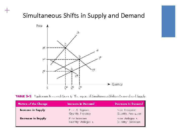
+ Simultaneous Shifts in Supply and Demand
Managerial Economics Chapter Two.pptx