8c8bd2d3863f1f26d9f33ebb2df4b5a2.ppt
- Количество слайдов: 170

Making Better Decisions Itzhak Gilboa 1
Judgment and Decision Biases 2
Problems 2. 1, 2. 12 A 65 -year old relative of yours suffers from a serious disease. It makes her life miserable, but does not pose an immediate risk to her life. She can go through an operation that, if successful, will cure her. However, the operation is risky. (A: 30% of the patients undergoing it die. B: 70% of the patients undergoing it survive. ) Would you recommend that she undergoes it? 3
Framing Effects • Representations matter • Implicitly assumed away in economic theory • Cash discount • Tax deductions • Formal models 4
Problems 2. 2, 2. 13 A: You are given $1, 000 for sure. Which of the following two options would you prefer? a. to get additional $500 for sure; b. to get another $1, 000 with probability 50%, and otherwise – nothing more (and be left with the first $1, 000 ). B: You are given $2, 000 for sure. Which of the following two options would you prefer? a. to lose $500 for sure; b. to lose $1, 000 with probability 50%, and otherwise – to lose nothing. 5
Problem 2. 2, 2. 13 In both versions the choice is between: a. $1, 500 for sure; b. $1, 000 with probability 50%, and $2, 000 with probability 50%. Framing 6
Gain-Loss Asymmetry • Loss aversion • Relative to a reference point • Risk aversion in the domain of gains, but evidence of loss aversion in the domain of losses 7
Is it rational to fear losses? Three scenarios: • The politician • The spouse • The self The same mode of behavior may be rational in some domains but not in others 8
Endowment Effect What’s the worth of a coffee mug? • How much would you pay to buy it? • What gift would be equivalent? • How much would you demand to sell it? Should all three be the same? 9
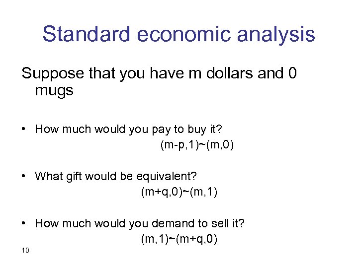
Standard economic analysis Suppose that you have m dollars and 0 mugs • How much would you pay to buy it? (m-p, 1)~(m, 0) • What gift would be equivalent? (m+q, 0)~(m, 1) • How much would you demand to sell it? (m, 1)~(m+q, 0) 10
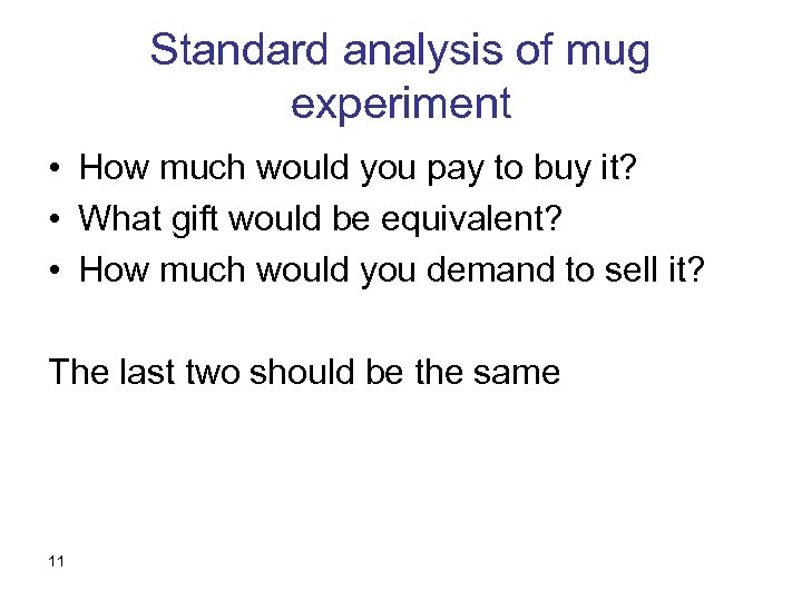
Standard analysis of mug experiment • How much would you pay to buy it? • What gift would be equivalent? • How much would you demand to sell it? The last two should be the same 11
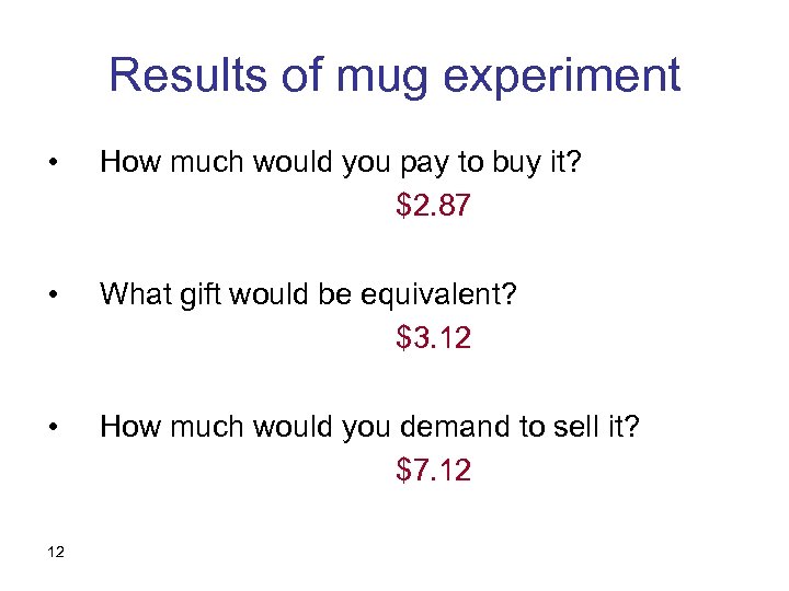
Results of mug experiment • How much would you pay to buy it? $2. 87 • What gift would be equivalent? $3. 12 • How much would you demand to sell it? $7. 12 12
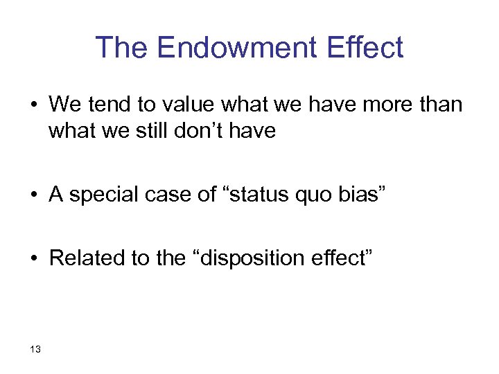
The Endowment Effect • We tend to value what we have more than what we still don’t have • A special case of “status quo bias” • Related to the “disposition effect” 13
Is it rational … to value a house your grandfather’s pen your car equity … just because it’s yours? 14
Rationalization of Endowment Effect • Information (used car) • Stabilization of choice • Habits and efficiency (word processor) 15
Problem 2. 3, 2. 14 • 2. 3: You go to a movie. It was supposed to be good, but it turns out to be boring. Would you leave in the middle and do something else instead? • 2. 14 reads: Your friend had a ticket to a movie. She couldn’t make it, and gave you the ticket “instead of just throwing it away”. The movie was supposed to be good, but it turns out to be boring. Would you leave in the middle and do something else instead? 16
Sunk Cost • Cost that is “sunk” should be ignored • Often, it’s not • Is it rational? 17
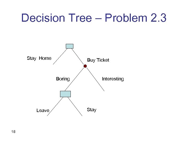
Decision Tree – Problem 2. 3 Stay Home Buy Ticket Boring Leave 18 Interesting Stay
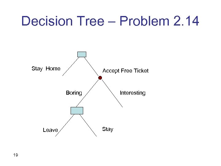
Decision Tree – Problem 2. 14 Stay Home Accept Free Ticket Boring Leave 19 Interesting Stay
Consequentialism • Only the consequences, or the rest of the tree, matter • Helps ignore sunk costs if we so wish • Does it mean we’ll be ungrateful to our old teachers? 20
Problem 2. 4, 2. 15 Linda is 31 years old… etc. How many ranked f. Linda is a bank teller Below h. Linda is a bank teller who is active in a feminist movement ? 21
Representativeness Heuristic The conjunction fallacy Many explanations: – “a bank teller” – “a bank teller who is not active”? – Ranking propositions is not a very natural task Still, the main point remains: heuristics can be misleading 22
Problems 2. 5, 2. 16 A: In four pages of a novel (about 2, 000 words) in English, do you expect to find more than ten words that have the form _ _ _n _ (sevenletter words that have the letter n in the sixth position)? B: In four pages of a novel (about 2, 000 words) in English, do you expect to find more than ten words that have the form _ _ ing (sevenletter words that end with ing)? 23
Availability Heuristic In the absence of a “scientific” database, we use our memory Typically, a great idea Sometimes, results in a biased sample 24
Problems 2. 6, 2. 17 A: What is the probability that, in the next 2 years, there will be a cure for AIDS? B: What is the probability that, in the next 2 years, there will be a new genetic discovery in the study of apes, and a cure for AIDS? Availability heuristic 25
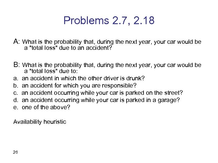
Problems 2. 7, 2. 18 A: What is the probability that, during the next year, your car would be a "total loss" due to an accident? B: What is the probability that, during the next year, your car would be a. b. c. d. e. a "total loss" due to: an accident in which the other driver is drunk? an accident for which you are responsible? an accident occurring while your car is parked on the street? an accident occurring while your car is parked in a garage? one of the above? Availability heuristic 26
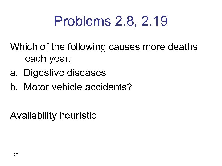
Problems 2. 8, 2. 19 Which of the following causes more deaths each year: a. Digestive diseases b. Motor vehicle accidents? Availability heuristic 27
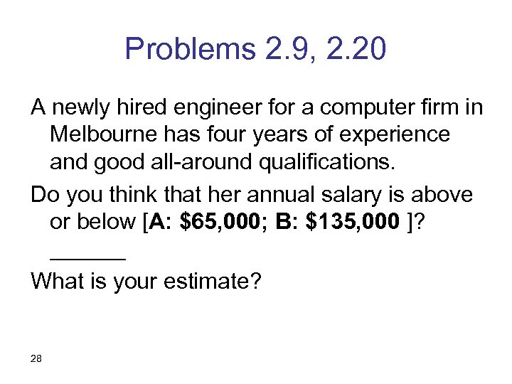
Problems 2. 9, 2. 20 A newly hired engineer for a computer firm in Melbourne has four years of experience and good all-around qualifications. Do you think that her annual salary is above or below [A: $65, 000; B: $135, 000 ]? ______ What is your estimate? 28
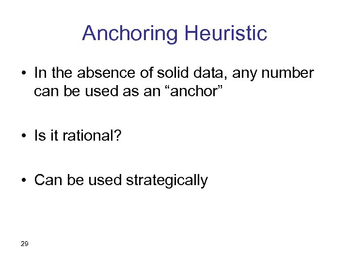
Anchoring Heuristic • In the absence of solid data, any number can be used as an “anchor” • Is it rational? • Can be used strategically 29
Problems 2. 10, 2. 21 • A: You have a ticket to a concert, which cost you $50. When you arrive at the concert hall, you find out that you lost the ticket. Would you buy another one (assuming you have enough money in your wallet)? • B: You are going to a concert. Tickets cost $50. When you arrive at the concert hall, you find out that you lost a $50 bill. Would you still buy the ticket (assuming you have enough money in your wallet)? 30
Mental Accounting • Different expenses come from “different” accounts. • Other examples: – Your spouse buys you the gift you didn’t afford – You spend more on special occasions (moving; travelling) – Driving to a game in the snow (wouldn’t do it if the tickets had been free) 31
Is it rational? Mental accounting can be useful: – Helps solve a complicated budget problem top -down – Helps cope with self-control problems – Uses external events as memory aids … but it can sometimes lead to decisions we won’t like (driving in the snow…) 32
Problems 2. 11, 2. 22 A: Which of the following two options do you • • prefer? Receiving $10 today. Receiving $12 a week from today. B: Which of the following two options do you prefer? • Receiving $10 50 weeks from today. • Receiving $12 51 weeks from today. 33
![Discounting • Classical: U(c 1, c 2, …) = [1/(1 - δ )] * Discounting • Classical: U(c 1, c 2, …) = [1/(1 - δ )] *](https://present5.com/presentation/8c8bd2d3863f1f26d9f33ebb2df4b5a2/image-34.jpg)
Discounting • Classical: U(c 1, c 2, …) = [1/(1 - δ )] * ∑i δi u(ci) -- violated in the example above. • Hyperbolic: more weight on period no. 1 34
Summary • Many of the classical economic assumptions are violated • Some violations are more rational than others • Formal models may help us decide which modes of behavior we would like to change 35
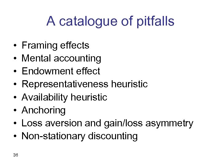
A catalogue of pitfalls • • 36 Framing effects Mental accounting Endowment effect Representativeness heuristic Availability heuristic Anchoring Loss aversion and gain/loss asymmetry Non-stationary discounting
Consuming Statistical Data 37
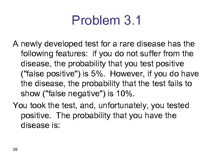
Problem 3. 1 A newly developed test for a rare disease has the following features: if you do not suffer from the disease, the probability that you test positive ("false positive") is 5%. However, if you do have the disease, the probability that the test fails to show ("false negative") is 10%. You took the test, and, unfortunately, you tested positive. The probability that you have the disease is: 38
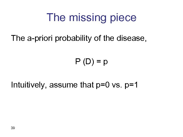
The missing piece The a-priori probability of the disease, P (D) = p Intuitively, assume that p=0 vs. p=1 39
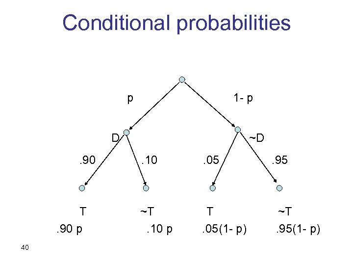
Conditional probabilities p 1 - p D. 90 T. 90 p 40 ~D. 10 . 05 ~T. 10 p T. 05(1 - p) . 95 ~T. 95(1 - p)
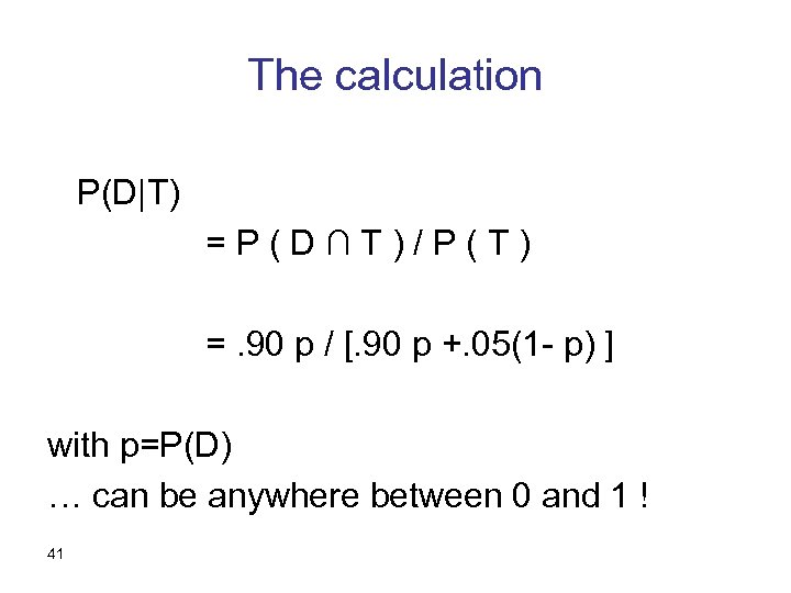
The calculation P(D|T) =P(D∩T)/P(T) =. 90 p / [. 90 p +. 05(1 - p) ] with p=P(D) … can be anywhere between 0 and 1 ! 41
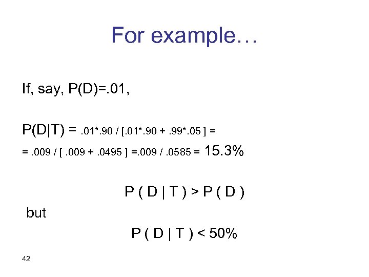
For example… If, say, P(D)=. 01, P(D|T) =. 01*. 90 / [. 01*. 90 +. 99*. 05 ] = =. 009 / [. 009 +. 0495 ] =. 009 /. 0585 = 15. 3% P(D|T)>P(D) but P ( D | T ) < 50% 42
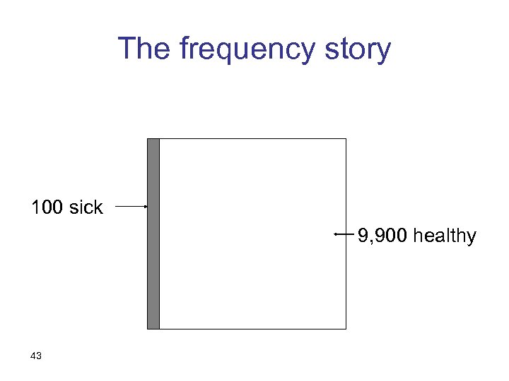
The frequency story 100 sick 9, 900 healthy 43
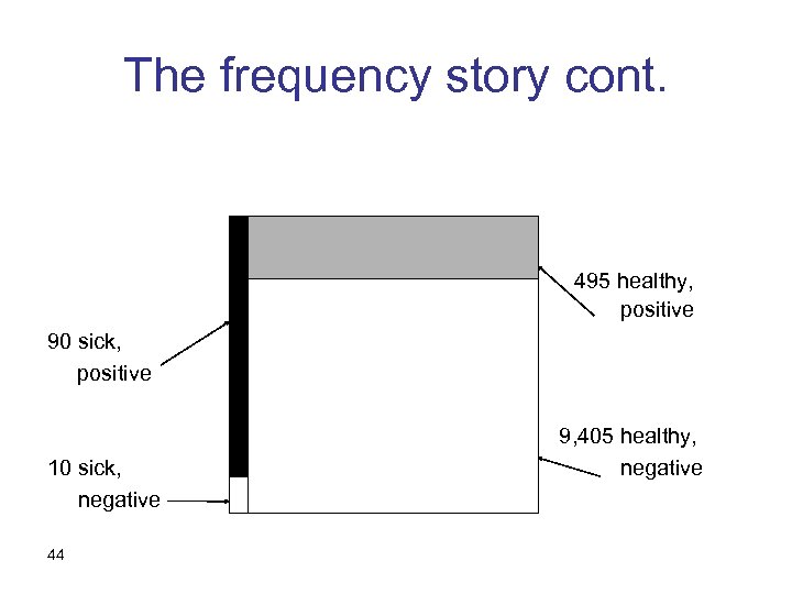
The frequency story cont. 495 healthy, positive 90 sick, positive 10 sick, negative 44 9, 405 healthy, negative
![Ignoring Base Probabilities P ( A | B ) = [P(A)/P(B)] P ( B Ignoring Base Probabilities P ( A | B ) = [P(A)/P(B)] P ( B](https://present5.com/presentation/8c8bd2d3863f1f26d9f33ebb2df4b5a2/image-45.jpg)
Ignoring Base Probabilities P ( A | B ) = [P(A)/P(B)] P ( B | A ) In general, P(B|A) ≠ P(A|B) 45
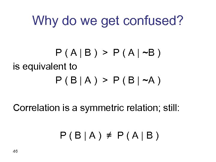
Why do we get confused? P ( A | B ) > P ( A | ~B ) is equivalent to P ( B | A ) > P ( B | ~A ) Correlation is a symmetric relation; still: P(B|A) ≠ P(A|B) 46
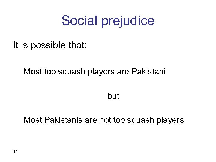
Social prejudice It is possible that: Most top squash players are Pakistani but Most Pakistanis are not top squash players 47
Problem 3. 2 You are going to play the roulette. You first sit there and observe, and you notice that the last five times it came up "black. " Would you bet on "red" or on "black"? 48
The Gambler’s Fallacy • If you believe that the roulette is fair, there is independence • By definition, you can learn nothing from the past about the future • Law of large numbers: errors do not get corrected, they get diluted. 49
Errors are “diluted” • Suppose we observe 1000 blacks • The prediction for the next 1, 000 will still be 500, 000 ; 500, 000 • Resulting in 501, 000 ; 500, 000 50
Maybe the roulette is not fair? • Indeed, we will have to conclude this after, say, 1, 000 blacks. • But then we will expect black, not red • We assume independence given the parameter of the roulette wheel, but we can learn from observations about this parameter 51
Problem 3. 3 • A study of students’ grades in the US showed that immigrants had, on average, a higher grade point average than did USborn students. The conclusion was that Americans are not very smart, or at least do not work very hard, as compared to other nationalities. 52
Biased Samples • The point: immigrants are not necessarily representative of the home population • The Literary Digest 1936 fiasco • Students who participate in class • Citizens who exercise the right to vote 53
Problem 3. 4 • In order to estimate the average number of children in a family, a researcher sampled children in a school, and asked them how many siblings they had. The answer, plus one, was averaged over all children in the sample to provide the desired estimate. 54
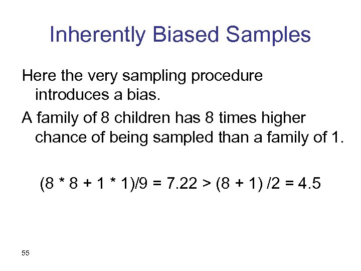
Inherently Biased Samples Here the very sampling procedure introduces a bias. A family of 8 children has 8 times higher chance of being sampled than a family of 1. (8 * 8 + 1 * 1)/9 = 7. 22 > (8 + 1) /2 = 4. 5 55
Problem 3. 5 • A contractor of small renovation projects submits bids and competes for contracts. He noticed that he tends to lose money on the projects he runs. He started wondering how he can be so systematically wrong in his estimates. 56
The Winner’s Curse • Firms that won auctions tended to lose money • Even if the estimate is unbiased ex-ante, it is not unbiased ex-post, given that one has one the auction. • If you won the auction, it is more likely that this was one of your over-estimates rather than one of your under-estimates. 57
Problem 3. 6 Ann: “Do you like your dish? ” Barbara: “Well, it isn’t bad. Maybe not as good as last time, but…” If the restaurant isn’t so new, how would you explain it? 58
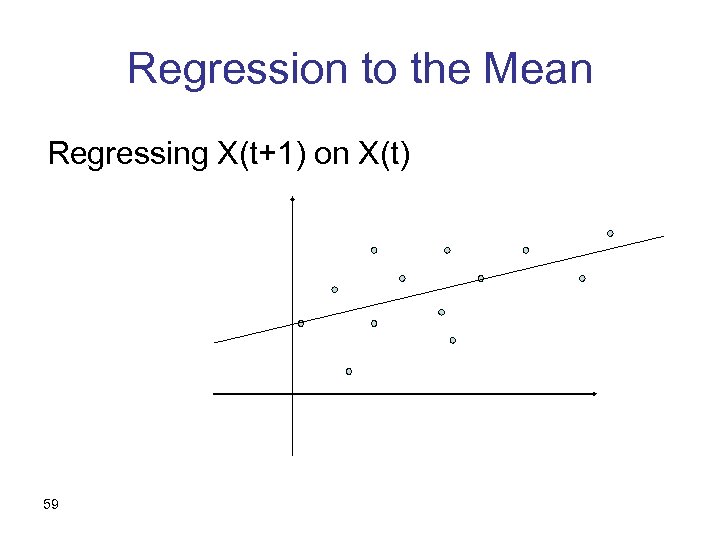
Regression to the Mean Regressing X(t+1) on X(t) 59
Regression to the Mean – cont. • We should expect an increasing line • We should expect a slope < 1 • Students selected by grades • Your friend’s must-see movie • Selection brokers; electing politicians 60
Problem 3. 7 Studies show a high correlation between years of education and annual income. Thus, argued your teacher, it’s good for you to study: the more you do, the more money you will make in the future. 61
Correlation and Causality Possible reasons for correlation between X and Y: • X is a cause of Y • Y is a cause of X • Z is a common cause of both X and Y • Coincidence (should be taken care of by statistical significance) 62
Problem 3. 8 • In a recent study, it was found that people who did not smoke at all had more visits to their doctors than people who smoked a little bit. One researcher claimed, “Apparently, smoking is just like consuming red wine – too much of it is dangerous, but a little bit is actually good for your health!” 63
Correlation and Causality – cont. Other examples: • Do hospitals make you sick? • Will a larger hand improve the child’s handwriting? 64
Problem 3. 9 Daniel: “Fine, it’s your decision. But I tell you, the effects that were found were insignificant. ” Charles: “Insignificant? They were significant at the 5% level!” 65
Statistical Significance • Means that the null hypothesis can be rejected, knowing that, if it were true, the probability of being rejected is quite low • Does not imply that the null hypothesis is wrong • Does not even imply that the probability of the null hypothesis is low 66
The mindset of hypotheses testing • We wish to prove a claim • We state as the null hypothesis, H 0, its negation • By rejection the negation, we will “prove” the claim 67
The mindset of hypotheses testing – cont. • A test is a rule, saying when to say “reject” based on the sample • Type I error: rejecting H 0 when it is, in fact, true • Type II error: failing to reject H 0 when it is, in fact, false 68
The mindset of hypotheses testing – cont. • What is the probability of type I error? – Zero if the null hypothesis is false – Typically unknown if it is true – Overall, never known. • So what is the significance level, α ? – The maximal probability possible (over all values consistent with the null hypothesis) 69
The mindset of hypotheses testing – cont. • We never state the probability of the null hypothesis being true • Neither before nor after taking the sample • This would depend on subjective judgment that we try to avoid 70
Problem 3. 10 Mary: “I don’t get it. It’s either or: if you’re so sure it’s OK, why isn’t it approved? If it’s not yet approved, it’s probably not yet OK. ” 71
Classical and Bayesian Statistics • Bayesian: – Quantify everything probabilistically – Take a prior, observe data, update to a posterior – Can treat an unknown parameter, µ, and the sample, X, on equal ground – A priori beliefs about the unknown parameter are updated by Bayes rule 72
Classical and Bayesian Statistics – cont. • Classical: – Probability exists only given the unknown parameter – There are no probabilistic beliefs about it – µ is a fixed number, though unknown – X is a random variable (known after the sample is taken) – Uses “confidence” and “significance”, which are not “probability” 73
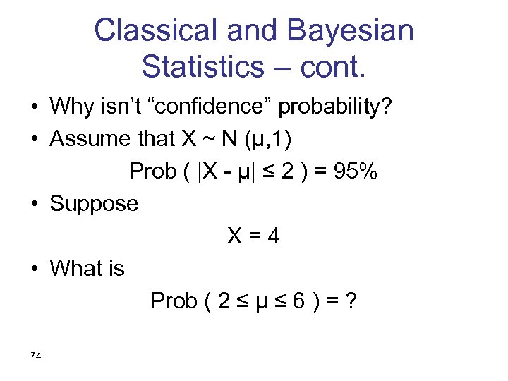
Classical and Bayesian Statistics – cont. • Why isn’t “confidence” probability? • Assume that X ~ N (µ, 1) Prob ( |X - µ| ≤ 2 ) = 95% • Suppose X=4 • What is Prob ( 2 ≤ µ ≤ 6 ) = ? 74
Classical and Bayesian Statistics – cont. • The question is ill-defined, because µ is not a random variable. Never has been, never will. • The statement Prob ( |X - µ| ≤ 2 ) = 95% is a probability statement about X, not about µ 75
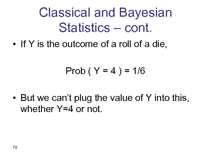
Classical and Bayesian Statistics – cont. • If Y is the outcome of a roll of a die, Prob ( Y = 4 ) = 1/6 • But we can’t plug the value of Y into this, whether Y=4 or not. 76
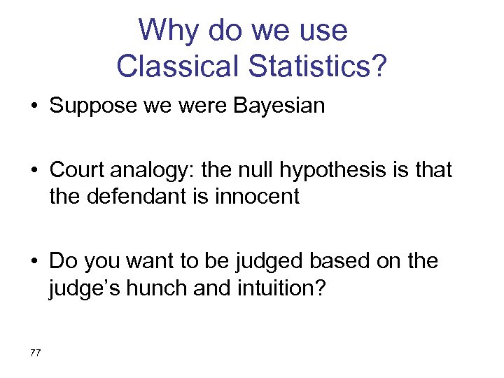
Why do we use Classical Statistics? • Suppose we were Bayesian • Court analogy: the null hypothesis is that the defendant is innocent • Do you want to be judged based on the judge’s hunch and intuition? 77
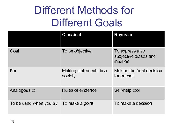
Different Methods for Different Goals Classical Bayesian Goal To be objective To express also subjective biases and intuition For Making statements in a society Making the best decision for oneself Analogous to Rules of evidence Self-help tool To be used when you try To make a point To make a decision 78
Decision Under Risk 79
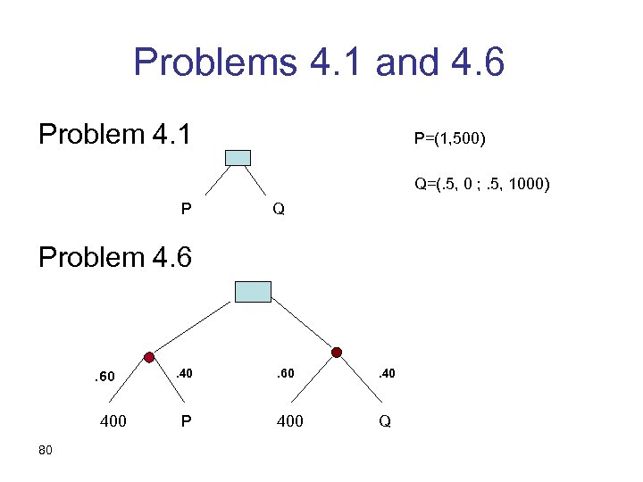
Problems 4. 1 and 4. 6 Problem 4. 1 P=(1, 500) Q=(. 5, 0 ; . 5, 1000) P Q Problem 4. 6 . 60 400 80 . 40 P . 60 . 40 400 Q
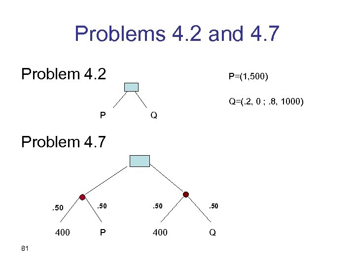
Problems 4. 2 and 4. 7 Problem 4. 2 P=(1, 500) Q=(. 2, 0 ; . 8, 1000) P Q Problem 4. 7 . 50 400 81 . 50 P . 50 400 Q
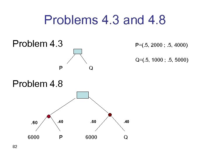
Problems 4. 3 and 4. 8 Problem 4. 3 P=(. 5, 2000 ; . 5, 4000) Q=(. 5, 1000 ; . 5, 5000) P Q Problem 4. 8 . 60 6000 82 . 40 P 6000 . 40 Q
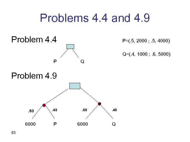
Problems 4. 4 and 4. 9 Problem 4. 4 P=(. 5, 2000 ; . 5, 4000) Q=(. 4, 1000 ; . 6, 5000) P Q Problem 4. 9 . 60 6000 83 . 40 P 6000 . 40 Q
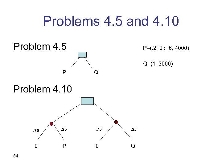
Problems 4. 5 and 4. 10 Problem 4. 5 P=(. 2, 0 ; . 8, 4000) Q=(1, 3000) P Q Problem 4. 10 . 75 0 84 . 25 P . 75 . 25 0 Q
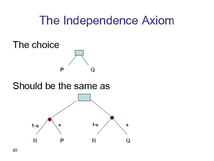
The Independence Axiom The choice P Q Should be the same as 1 -α R 85 α P 1 -α α R Q
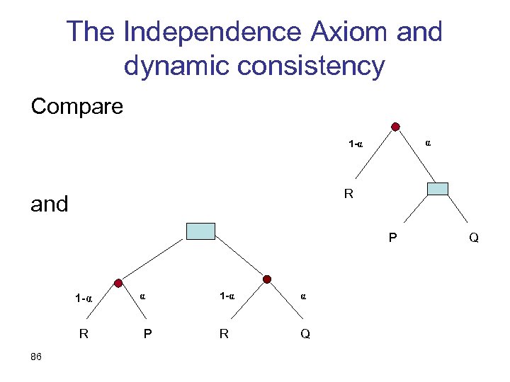
The Independence Axiom and dynamic consistency Compare α 1 -α R and P 1 -α R 86 α P 1 -α α R Q Q
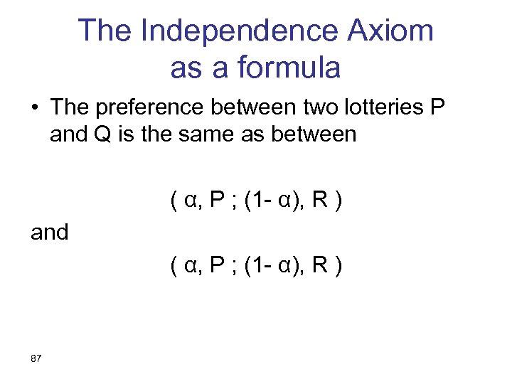
The Independence Axiom as a formula • The preference between two lotteries P and Q is the same as between ( α, P ; (1 - α), R ) and ( α, P ; (1 - α), R ) 87
von-Neumann Morgenstern’s Theorem • A preference order ≥ over lotteries (with known probabilities) satisfies: – Weak order (complete and transitive) – Continuity – Independence IF AND ONLY IF • It can be represented by the maximization of the expectation of a “utility” function 88
Expected Utility • Suggested by Daniel Bernoulli in the 18 th century • A lottery (p 1, x 1; … ; pn, xn) is evaluated by the expectation of the utility: p 1*u(x 1) + … + pn*u(xn) 89
Implications of the Theorem • Descriptively: it is perhaps reasonable that maximization of expected utility is a good model of people’s behavior • Normatively: Maybe we would like to maximize expected utility even if we don’t do it anyway 90
Calibration of Utility • If we believe that a decision maker is an EU maximizer, we can calibrate her utility function by asking, for which p is ( 1, $500 ) Equivalent to ( (1 -p), $0 ; p, $1, 000 ) 91
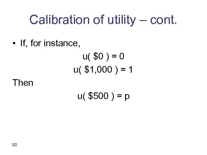
Calibration of utility – cont. • If, for instance, u( $0 ) = 0 u( $1, 000 ) = 1 Then u( $500 ) = p 92
Problem 4. 1 • Do you prefer $500 for sure or (. 50, $0 ; . 50, $1, 000 ) ? • Preferring 500 for sure indicates risk aversion. • Defined as preferring E(X) to X for any random variable X. 93
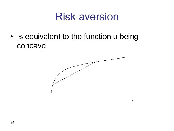
Risk aversion • Is equivalent to the function u being concave 94
Ample evidence that • The independence axiom fails in examples such as 4. 5 and 4. 10. • Why? • A version of Allais’ paradox • Kahneman and Tversky: Certainty Effect 95
Do People Satisfy the Independence Axiom? • Compare your choices in problems 4. 5 and 4. 10. • The Independence Axiom suggests that you make the same choices in both. 96
Another example • Do you prefer $1, 000 with probability 0. 8 or $2, 000 with probability 0. 4 ? • How about $1, 000 with probability 0. 0008 or $2, 000 with probability 0. 0004 ? 97
Prospect Theory Two main components: • People exhibit gain-loss asymmetry • People “distort” probabilities 98
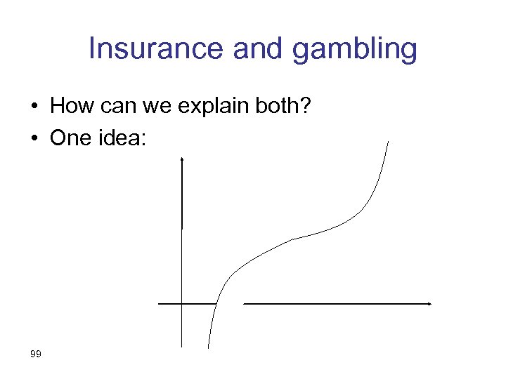
Insurance and gambling • How can we explain both? • One idea: 99
Insurance and gambling – cont. • How come all these people around the inflection point of their utility function? • To be honest, it’s not clear that the outcomes are properly defined • Yet: maybe the inflection point moves around with their wealth? 100
Gain-Loss Asymmetry • Positive-negative asymmetry in psychology • A “reference point” relative to which outcomes are defined • “Prospects” as opposed to “lotteries” 101
Probability Distortion • Small probabilities appear larger than they are in terms of their “decision weights” • State lotteries and insurance • A probability distortion function – (Different for losses and for gains) 102
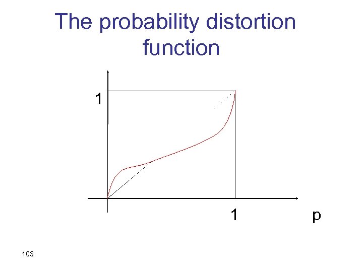
The probability distortion function 1 1 103 p
Decision Under Uncertainty 104
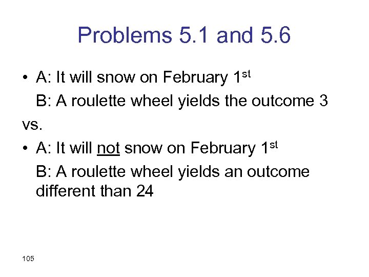
Problems 5. 1 and 5. 6 • A: It will snow on February 1 st B: A roulette wheel yields the outcome 3 vs. • A: It will not snow on February 1 st B: A roulette wheel yields an outcome different than 24 105
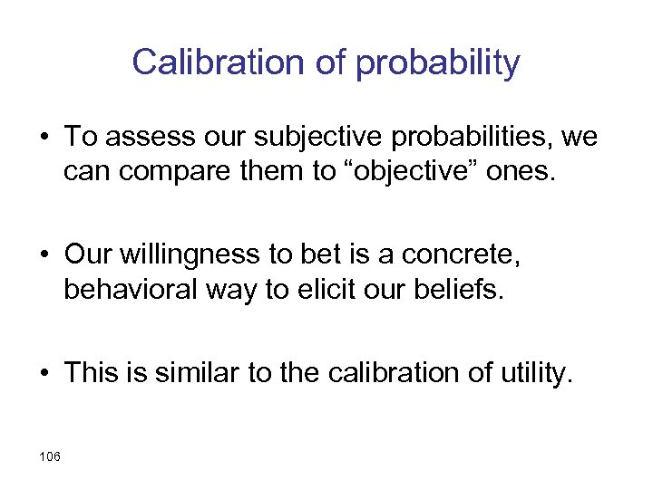
Calibration of probability • To assess our subjective probabilities, we can compare them to “objective” ones. • Our willingness to bet is a concrete, behavioral way to elicit our beliefs. • This is similar to the calibration of utility. 106
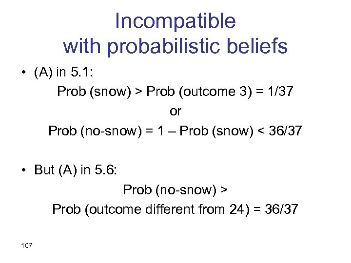
Incompatible with probabilistic beliefs • (A) in 5. 1: Prob (snow) > Prob (outcome 3) = 1/37 or Prob (no-snow) = 1 – Prob (snow) < 36/37 • But (A) in 5. 6: Prob (no-snow) > Prob (outcome different from 24) = 36/37 107
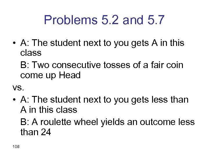
Problems 5. 2 and 5. 7 • A: The student next to you gets A in this class B: Two consecutive tosses of a fair coin come up Head vs. • A: The student next to you gets less than A in this class B: A roulette wheel yields an outcome less than 24 108
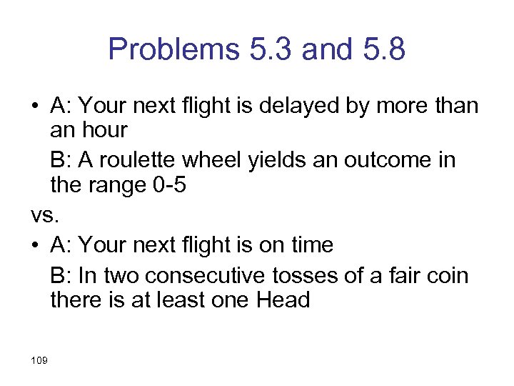
Problems 5. 3 and 5. 8 • A: Your next flight is delayed by more than an hour B: A roulette wheel yields an outcome in the range 0 -5 vs. • A: Your next flight is on time B: In two consecutive tosses of a fair coin there is at least one Head 109
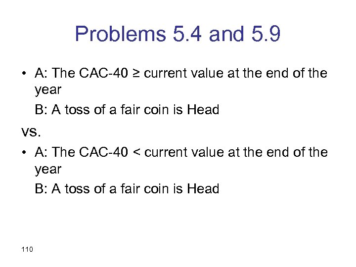
Problems 5. 4 and 5. 9 • A: The CAC-40 ≥ current value at the end of the year B: A toss of a fair coin is Head vs. • A: The CAC-40 < current value at the end of the year B: A toss of a fair coin is Head 110
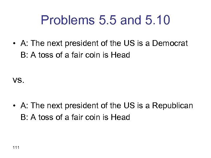
Problems 5. 5 and 5. 10 • A: The next president of the US is a Democrat B: A toss of a fair coin is Head vs. • A: The next president of the US is a Republican B: A toss of a fair coin is Head 111
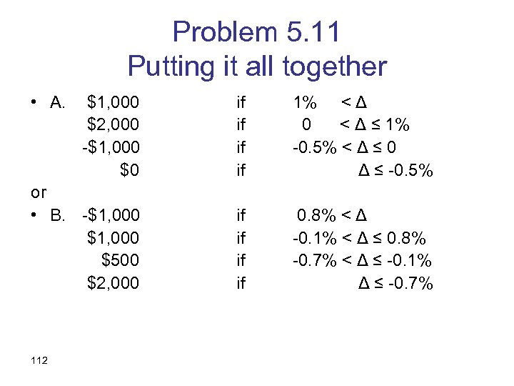
Problem 5. 11 Putting it all together • A. $1, 000 $2, 000 -$1, 000 $0 if if 1% < Δ 0 < Δ ≤ 1% -0. 5% < Δ ≤ 0 Δ ≤ -0. 5% or • B. -$1, 000 $500 $2, 000 if if 0. 8% < Δ -0. 1% < Δ ≤ 0. 8% -0. 7% < Δ ≤ -0. 1% Δ ≤ -0. 7% 112
Problem 5. 12 • First, let’s convince ourselves that “switch” wins with probability 2/3. • Suppose we named door A. • If the car really is behind A, we lost. • If the car is behind B, Monty opens C. “Switching” means “switching to B” and we win. • Similarly if the car is behind C. 113
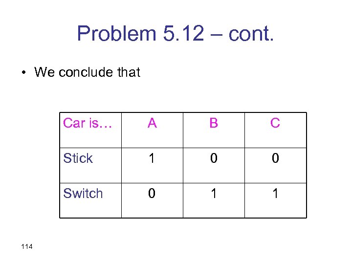
Problem 5. 12 – cont. • We conclude that Car is… B C Stick 1 0 0 Switch 114 A 0 1 1
Problem 5. 12 – cont. • To be convinced: – Assume that there were 1000 doors (and he has to open 998) – Realize that “switching” is not always to the same door – Monty Hall “helps” us by ruling out one of the bad choices we could have made. 115
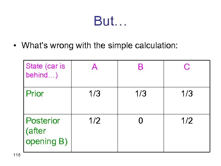
But… • What’s wrong with the simple calculation: State (car is behind…) B C Prior 1/3 1/3 Posterior (after opening B) 116 A 1/2 0 1/2
The problem • The state space above {A, B, C} is not rich enough • Assumptions that are hidden in the definition of the states will never be challenged by Bayesian updating • In particular, the way we get information, and the fact that we know something, may be informative in itself. 117
A correct Bayesian analysis • Suppose we named door A • Two sources of uncertainty – Where the car really is – Which door Monty Hall opens • Thus, there are 9 states of the world, not 3: 118
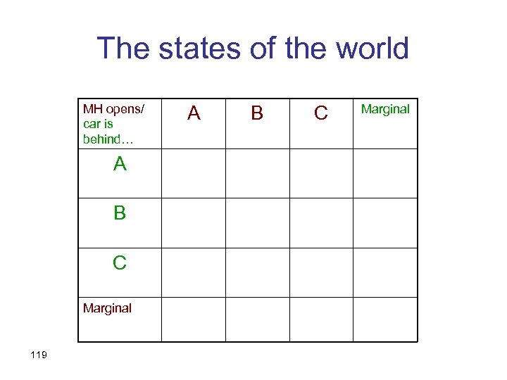
The states of the world MH opens/ car is behind… A B C Marginal 119 A B C Marginal
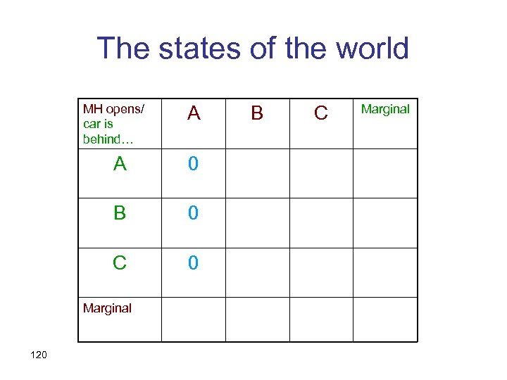
The states of the world MH opens/ car is behind… A A 0 B 0 C 0 Marginal 120 B C Marginal
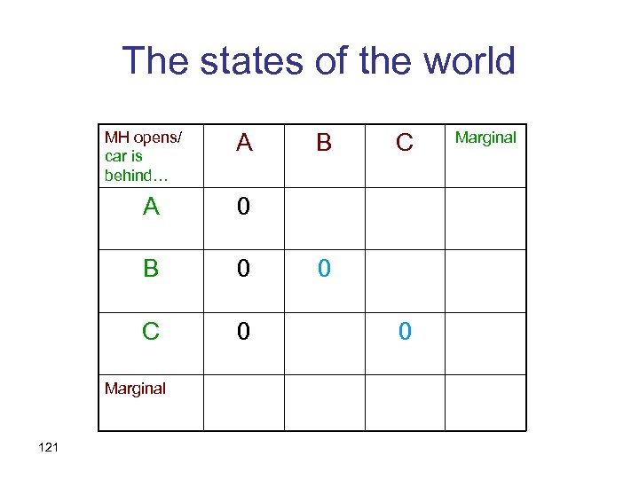
The states of the world MH opens/ car is behind… A A 0 C 0 Marginal 121 C 0 B B 0 0 Marginal
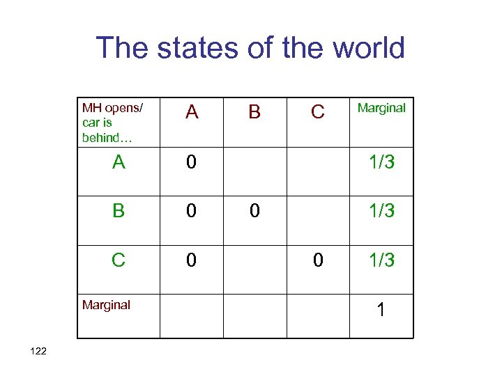
The states of the world MH opens/ car is behind… A A 0 C 0 Marginal 122 C 0 B B Marginal 1/3 0 1/3 1
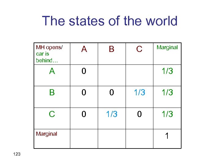
The states of the world MH opens/ car is behind… A B C Marginal A 0 B 0 0 1/3 C 0 1/3 Marginal 123 1/3 1
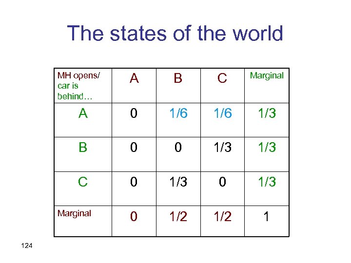
The states of the world MH opens/ car is behind… A B C Marginal A 0 1/6 1/3 B 0 0 1/3 C 0 1/3 0 1/2 1 Marginal 124
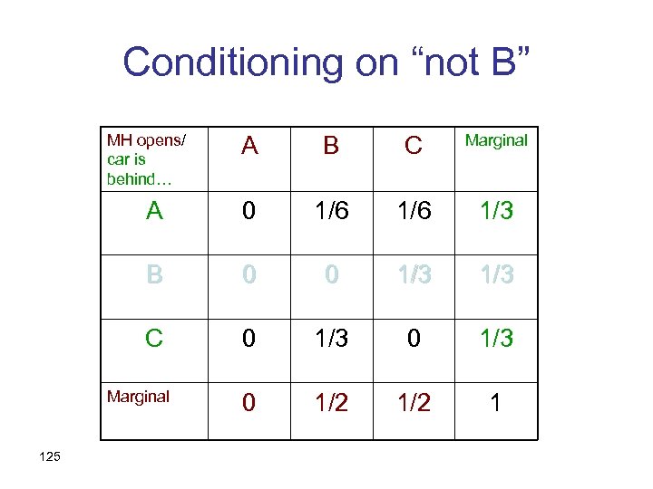
Conditioning on “not B” MH opens/ car is behind… A B C Marginal A 0 1/6 1/3 B 0 0 1/3 C 0 1/3 0 1/2 1 Marginal 125
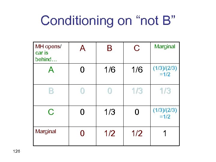
Conditioning on “not B” MH opens/ car is behind… A B C Marginal A 0 1/6 (1/3)/(2/3) =1/2 B 0 0 1/3 C 0 1/3 0 (1/3)/(2/3) =1/2 0 1/2 1 Marginal 126
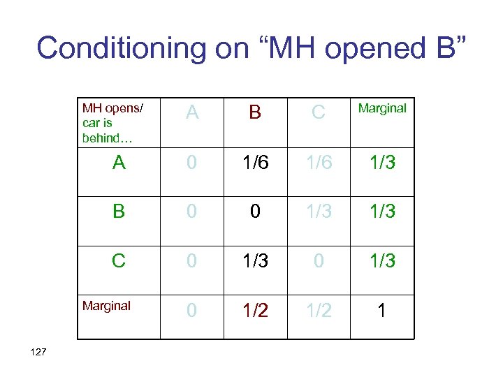
Conditioning on “MH opened B” MH opens/ car is behind… A B C Marginal A 0 1/6 1/3 B 0 0 1/3 C 0 1/3 0 1/2 1 Marginal 127
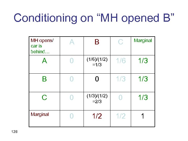
Conditioning on “MH opened B” MH opens/ car is behind… A B C Marginal A 0 (1/6)/(1/2) =1/3 1/6 1/3 B 0 0 1/3 C 0 (1/3)/(1/2) =2/3 0 1/2 1 Marginal 128
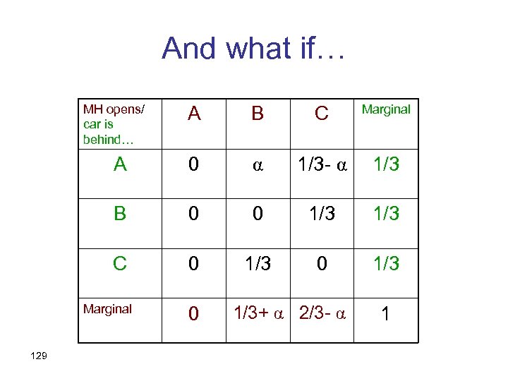
And what if… MH opens/ car is behind… A B C Marginal A 0 α 1/3 - α 1/3 B 0 0 1/3 C 0 1/3 Marginal 129 0 1/3+ α 2/3 - α 1
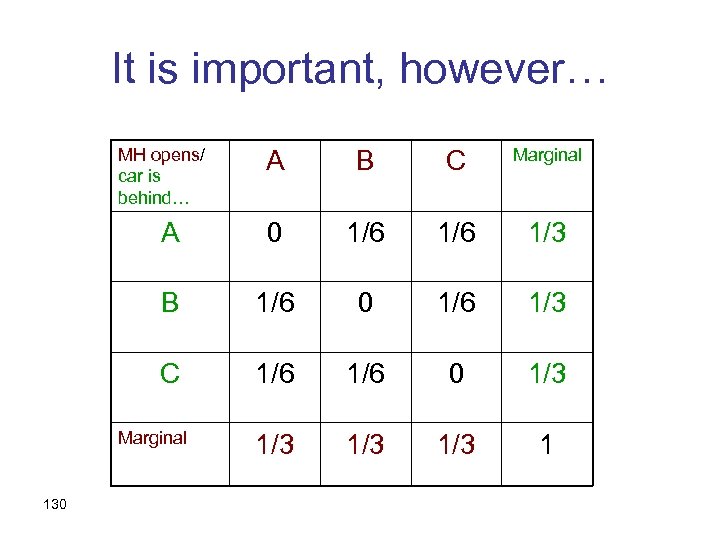
It is important, however… MH opens/ car is behind… A B C Marginal A 0 1/6 1/3 B 1/6 0 1/6 1/3 C 1/6 0 1/3 1/3 1 Marginal 130
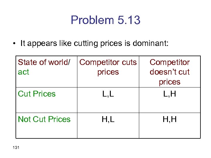
Problem 5. 13 • It appears like cutting prices is dominant: State of world/ act Cut Prices L, L Competitor doesn’t cut prices L, H Not Cut Prices H, L H, H 131 Competitor cuts prices
And yet… • Would you do it for real money? • If not, how would you justify it? 132
An alternative analysis • The states of the world should reflect all possible causal relationships • In order to assume nothing a-priori, we define states as functions from acts to outcomes: 133
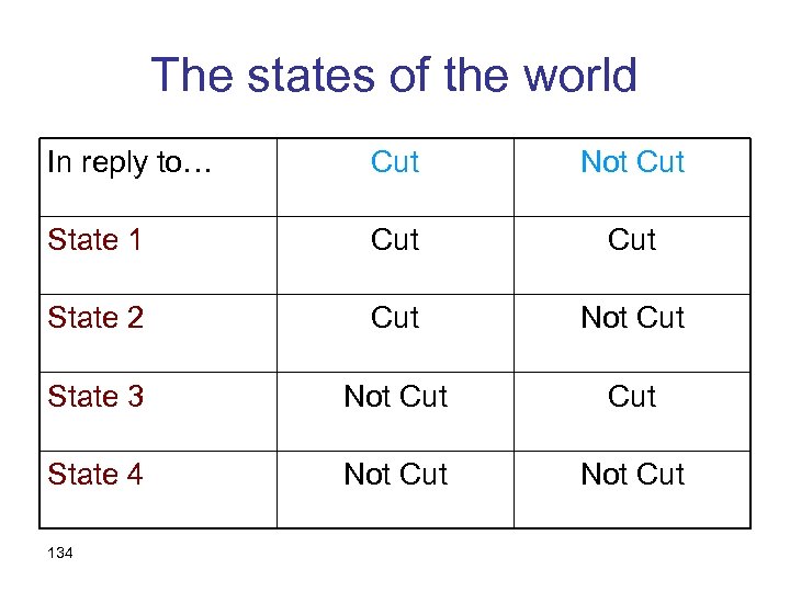
The states of the world In reply to… Cut Not Cut State 1 Cut State 2 Cut Not Cut State 3 Not Cut State 4 Not Cut 134
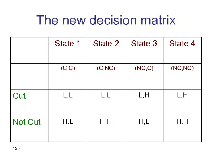
The new decision matrix State 1 State 2 State 3 State 4 (C, C) (C, NC) (NC, NC) Cut L, L L, H Not Cut H, L H, H 135
Important lessons • The states of the world should specify all the information that might be relevant, including how information was given. • The states of the world should allow for all causal relationships. • Other examples: political discussions 136
Problem 5. 14 (Ellsberg’s Two-Urn Paradox) • How many exhibit any preference between betting on Urn A vs. Urn B? • Of those – which did you prefer? 137
Evidence • A significant proportion of decision makers prefer to bet with known probabilities rather than with unknown ones. • Knight (1921) distinguished “risk” from “uncertainty” • Uncertainty/Ambiguity aversion 138
Problem 5. 15 (Ellsberg’s Single-Urn Paradox) • Many prefer betting on red to betting on blue (or yellow) • But also betting on not-red to betting on not-blue (or not-yellow) • In both cases, the bets defined by red have known probabilities, as opposed to those defined by blue (or yellow) 139
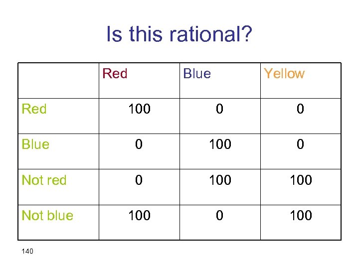
Is this rational? Red Blue Yellow Red 100 0 0 Blue 0 100 0 Not red 0 100 Not blue 100 0 100 140
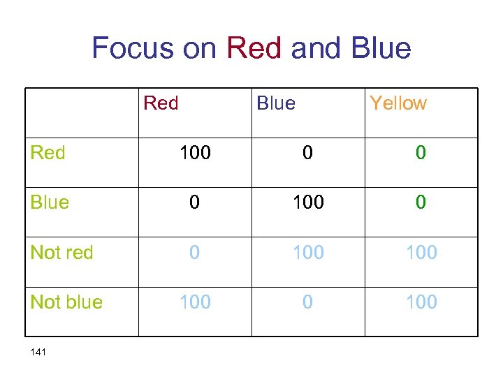
Focus on Red and Blue Red Blue Yellow Red 100 0 0 Blue 0 100 0 Not red 0 100 Not blue 100 0 100 141
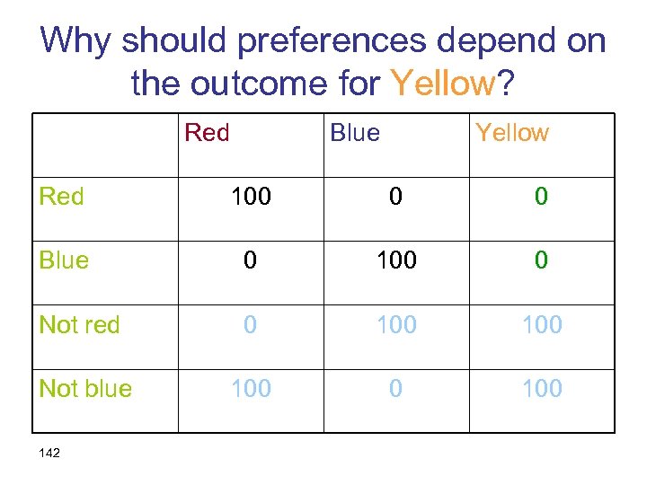
Why should preferences depend on the outcome for Yellow? Red Blue Yellow Red 100 0 0 Blue 0 100 0 Not red 0 100 Not blue 100 0 100 142
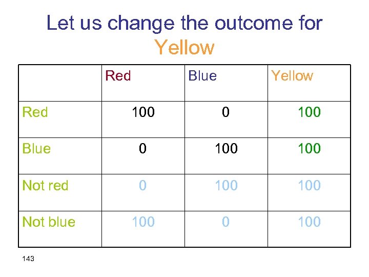
Let us change the outcome for Yellow Red Blue Yellow Red 100 0 100 Blue 0 100 Not red 0 100 Not blue 100 0 100 143
The Sure Thing Principle (Savage) • We compare acts, which are functions from states of the world to outcomes • If two acts are equal on a certain event, A, then the preferences between them should only depend on their values off A (on ~A). • Or: if we change them on A, but keep them equal to each other on A, preferences between them shouldn’t change. 144
Back to Problem 5. 14 • In order to see that the Sure Thing Principle is violated in this problem, we first have to define the state space • Recall that states assign outcomes to acts • From each urn we may draw either a red or a black ball • Hence there are four states of the world: 145
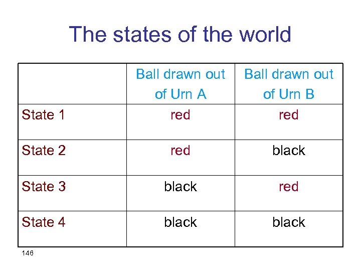
The states of the world State 1 Ball drawn out of Urn A red Ball drawn out of Urn B red State 2 red black State 3 black red State 4 black 146
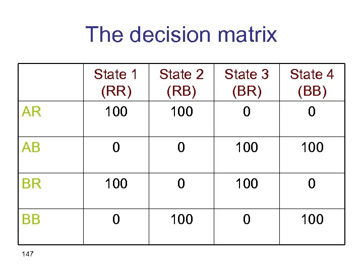
The decision matrix AR State 1 (RR) 100 State 2 (RB) 100 State 3 (BR) 0 State 4 (BB) 0 AB 0 0 100 BR 100 0 BB 0 100 147
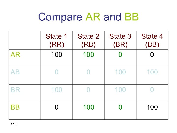
Compare AR and BB AR State 1 (RR) 100 State 2 (RB) 100 State 3 (BR) 0 State 4 (BB) 0 AB 0 0 100 BR 100 0 BB 0 100 148
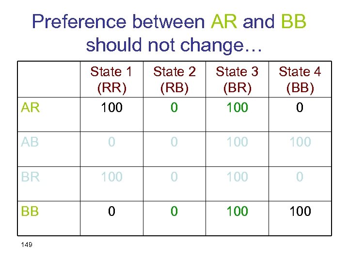
Preference between AR and BB should not change… AR State 1 (RR) 100 State 2 (RB) 0 State 3 (BR) 100 State 4 (BB) 0 AB 0 0 100 BR 100 0 BB 0 0 100 149
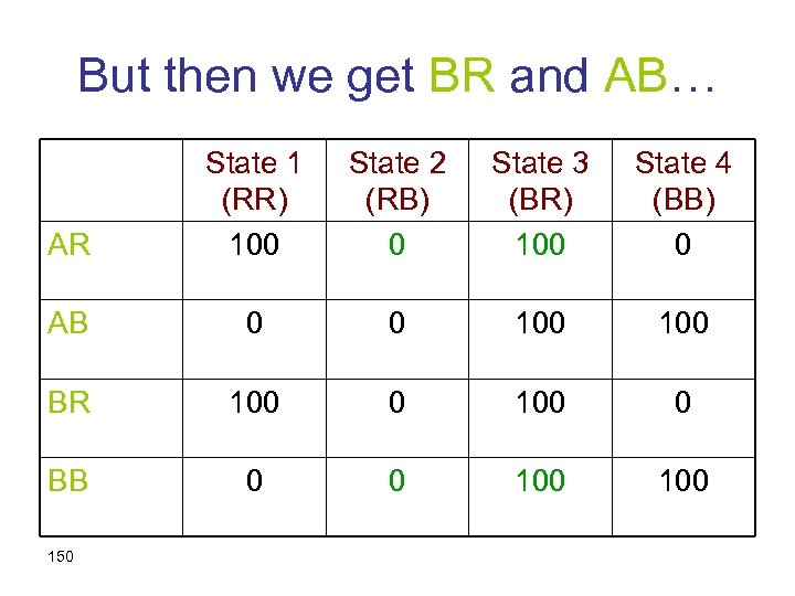
But then we get BR and AB… AR State 1 (RR) 100 State 2 (RB) 0 State 3 (BR) 100 State 4 (BB) 0 AB 0 0 100 BR 100 0 BB 0 0 100 150
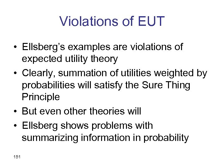
Violations of EUT • Ellsberg’s examples are violations of expected utility theory • Clearly, summation of utilities weighted by probabilities will satisfy the Sure Thing Principle • But even other theories will • Ellsberg shows problems with summarizing information in probability 151
Realistic examples • • 152 … are even more complicated Ellsberg’s urns have symmetries Real life often doesn’t The basic lesson: often we don’t have enough probability to generate a probabilistic belief
So what do we do? • One alternative: have a set of priors instead of one • How do we make decisions with a set of priors? 153
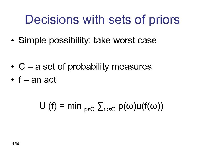
Decisions with sets of priors • Simple possibility: take worst case • C – a set of probability measures • f – an act U (f) = min pεC ∑ωεΩ p(ω)u(f(ω)) 154
Comments • The minimum reflects uncertainty aversion • It might be extreme and you can use other alternatives • In particular, using a set C which is a subset of the probability measures actually possible (based on your information). 155

Comments • The minimum reflects uncertainty aversion • It might be extreme and you can use other alternatives • In particular, using a set C which is a subset of the probability measures actually possible (based on your information). 156
Problem 5. 16 • How can my doctor figure out the probability of success in my case? • Aren’t we all different? 157
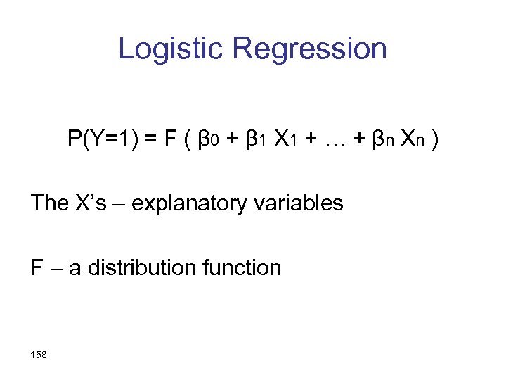
Logistic Regression P(Y=1) = F ( β 0 + β 1 X 1 + … + βn Xn ) The X’s – explanatory variables F – a distribution function 158
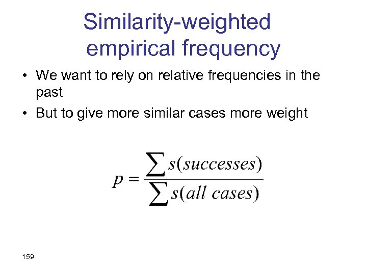
Similarity-weighted empirical frequency • We want to rely on relative frequencies in the past • But to give more similar cases more weight 159
Extreme special cases • All past cases equally similar – simple empirical frequency • Only identical cases are similar to degree 1 (others – 0) – conditional empirical frequency 160
Problem 5. 17 • But what about war? • As in the medical example, each case is different • A new problem: cases are not causally independent. 161
Well Being and Happiness 162
Problem 6. 1 and 6. 4 • Mary’s direct boss just quit, and you’re looking for someone for the job. You don’t think that Mary is perfect for it. By contrast, Jane seems a great fit. But it may be awkward to promote Jane and make Mary her subordinate. A colleague suggested that you go ahead and do this, but give both of them a nice raise to solve the problem. 163
Money and Well-Being • Money isn’t everything – Low correlation between income and wellbeing – The relative income hypothesis – Higher correlation within a cohort than across time – Relative to aspiration level 164
Other Determinants of Well-Being • Love, friendship • Social status • Self fulfillment – So how should we measure “success”? 165
Problem 6. 2 • As we’re nearing the end of this book, it is time to get some feedback. Please answer the following questions: • Did you find the explanations clear? • Did you find the topics interesting? • Did you find the graphs well done? • On a scale of 0 -10, your overall evaluation for the book is: 166
Problem 6. 5 • As we’re nearing the end of this book, it is time to get some feedback. Please answer the following questions: • On a scale of 0 -10, your overall evaluation for the book is: • Did you find the explanations clear? • Did you find the topics interesting? • Did you find the graphs well done? 167
Subjective Well Being • A common measure • Prone to manipulations – Dates and overall well-being – The weather: “deducting” irrelevant effects • Kahnemans’ Day Reconstruction Method 168
Problems 6. 3 and 6. 6 Robert is on a ski vacation with his wife, while John is at home. He can’t even dream of a ski vacation with the two children, to say nothing of the expense. In fact, John would be quite happy just to have a good night sleep. Do you think that Robert is happier than John? 169
What’s Happiness? • Both subjective well being and day reconstruction would suggest that Robert is happier • And yet… • What’s happiness for you? • How should we measure happiness for social policies? 170
8c8bd2d3863f1f26d9f33ebb2df4b5a2.ppt