Main Effects Screening A Distributed Continuous Quality Assurance

Main Effects Screening: A Distributed Continuous Quality Assurance Process for Monitoring Performance Degradation in Evolving Software Systems Cemal Yilmaz, Arvind S. Krishnaz, Atif Memon, Adam Porter, Douglas C. Schmidt, Aniruddha Gokhale, Balachandran Natarajan Presented By: Walaa El-Din M. Moustafa

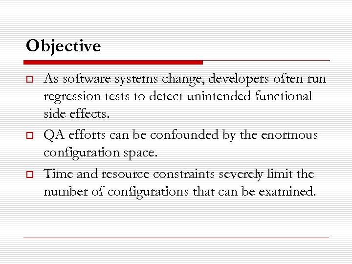
Objective o o o As software systems change, developers often run regression tests to detect unintended functional side effects. QA efforts can be confounded by the enormous configuration space. Time and resource constraints severely limit the number of configurations that can be examined.

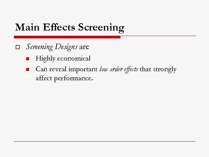
Main Effects Screening o Screening Designs are n n Highly economical Can reveal important low order effects that strongly affect performance.

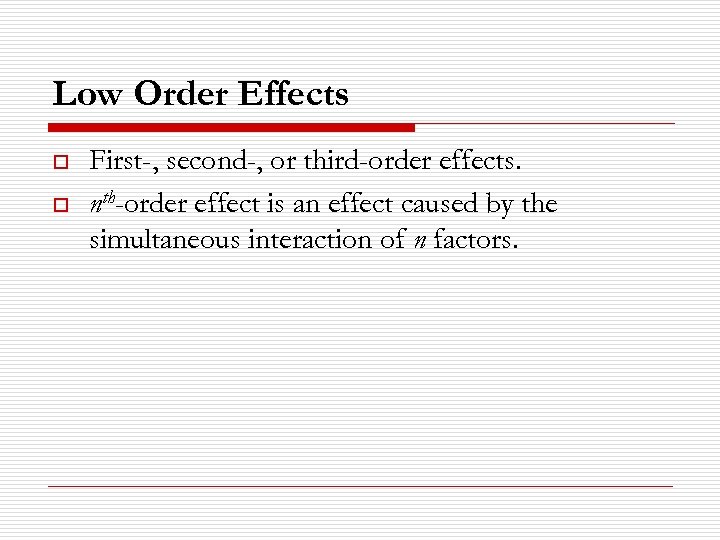
Low Order Effects o o First-, second-, or third-order effects. nth-order effect is an effect caused by the simultaneous interaction of n factors.

Low Order Effects Example o For certain web server applications: n n A 1 st-order effect might be that performance slows considerably when logging is turned on and another might be that it also slows when few server threads are used. A 2 nd order effect involves the interaction of two options, e. g. , web server performance may slow down when caching is turned off and the server performs blocking reads.

Factorial Designs o o Full factorial design involving k binary factors. Such a design exhaustively tests all combinations. Fractional factorial designs. These designs use only a carefully selected fraction (such as 1/2 or 1/4) of a full factorial design.

Fractional Factorial Designs o o Save money Do so by giving up the ability to measure some higher-order effects.

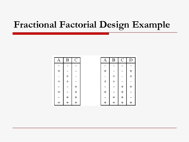
Fractional Factorial Design Example o To show screening designs are computed, we present a hypothetical example of a performance-intensive software system: n n n 4 binary configuration options, A through D. No inter-option constraints. The full configuration space therefore has 24 = 16 configurations.

Fractional Factorial Design Example o o o 8 configurations. Will focus only on 1 st-order effects. This design is referred to as a 24 -1 design, where 4 refers to the total number of options we will examine and the -1 (2 -1 = 1/2) indicates the fraction of the full factorial over which we will collect data.

Fractional Factorial Design Example o We can extend the design and estimate the effect of option D without going to a 24 full factorial design.

Fractional Factorial Design Example o Design Generator: n n Specifies the aliasing patterns used to build the design For this example, we select the design generator D = ABC.

Fractional Factorial Design Example

Fractional Factorial Design Example o o The design we described above is a resolution IV design. In resolution R designs, no effects involving i factors are aliased with effects involving less than R - i factors.

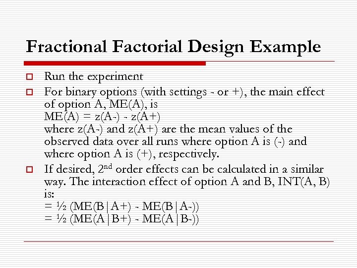
Fractional Factorial Design Example o o o Run the experiment For binary options (with settings - or +), the main effect of option A, ME(A), is ME(A) = z(A-) - z(A+) where z(A-) and z(A+) are the mean values of the observed data over all runs where option A is (-) and where option A is (+), respectively. If desired, 2 nd order effects can be calculated in a similar way. The interaction effect of option A and B, INT(A, B) is: = ½ (ME(B|A+) - ME(B|A-)) = ½ (ME(A|B+) - ME(A|B-))

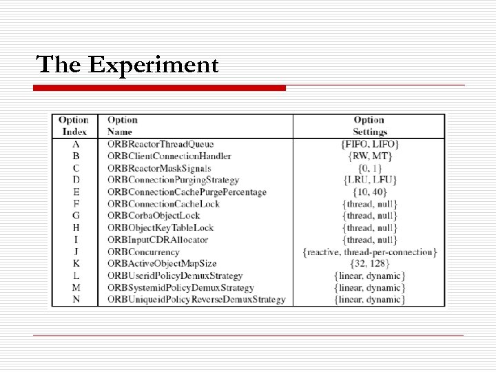
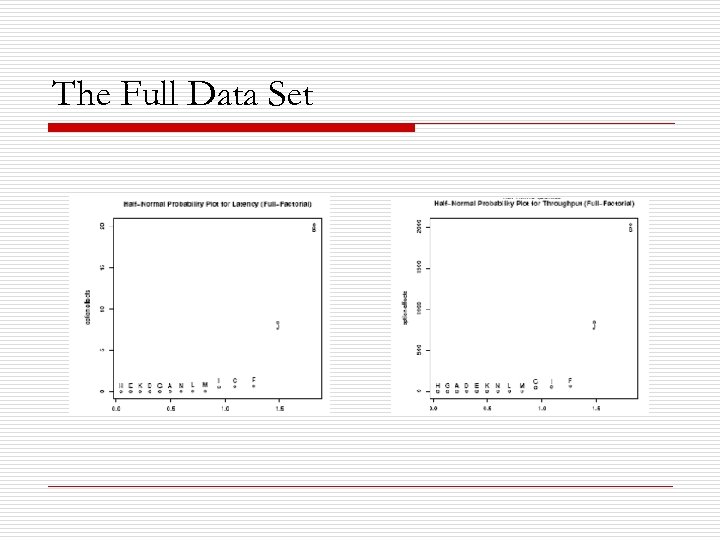
The Experiment o o o ACE v 5. 4 + TAO v 1. 4 + CIAO v 0. 4. 14 binary run-time options 214 = 16, 384 different configurations. For each task measure: n n Message latency. Throughput between the client and the server.

The Experiment

The Full Data Set

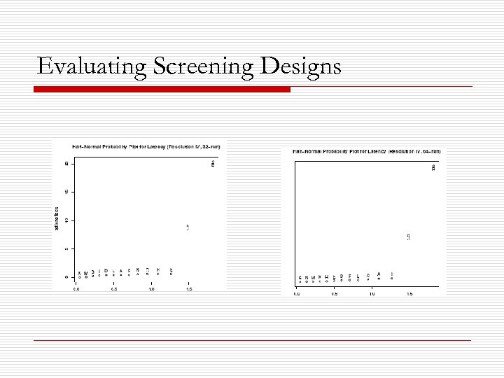
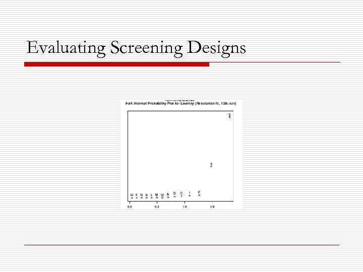
Evaluating Screening Designs o Can screening designs correctly identify the important options discovered during the analysis of the full data set?

Evaluating Screening Designs o o o Scr 32 is a 214 - 9 IV with design generators F = ABC, G = ABD, H = ACD, I = BCD, J = ABE, K = ACE, L = BCE, M = ADE, N = BDE. Scr 64 is a 214 - 8 IV with design generators G = ABC, H = ABD, I = ABE, J = ACDE, K = ABF, L = ACDF, M = ACEF, N = ADEF. Scr 128 is a 214 - 7 IV with design generators H = ABC, I = ABDE, J = ABDF, K = ACEF, L = ACDG, M = ABEFG, N = BCDEFG.

Evaluating Screening Designs

Evaluating Screening Designs o o Screening designs can detect important options at a large fraction of the cost of exhaustive testing. The smaller the effect, the larger the run size needed to identify it.

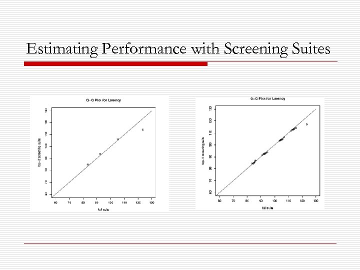
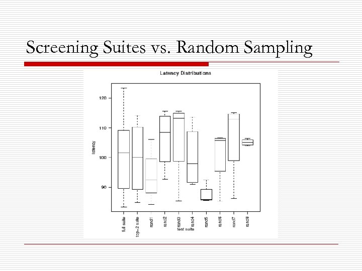
Estimating Performance with Screening Suites o o The estimates are generated by examining all combinations of the most important options, while defaulting the settings of the unimportant options Make the estimates based on benchmarking either 4 (all combinations of options B and J) or 32 (all combinations of options B, J, C, I, and F) configurations.

Estimating Performance with Screening Suites

Estimating Performance with Screening Suites o The distributions of the top-5 and top-2 screening suites closely track the overall performance data.

Screening Suites vs. Random Sampling

Screening Suites vs. Random Sampling o These graphs suggest the obvious weakness of random sampling.

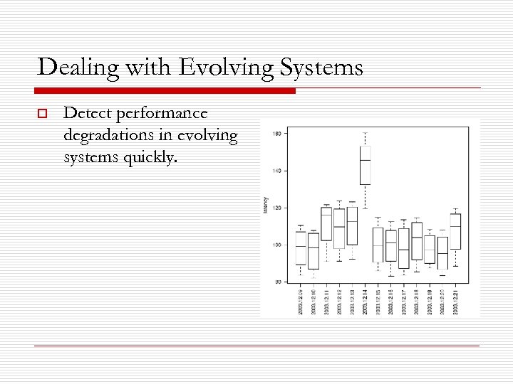
Dealing with Evolving Systems o Detect performance degradations in evolving systems quickly.

Dealing with Evolving Systems o Developer records and problem reports indicate that problems were noticed on 12/14/03.

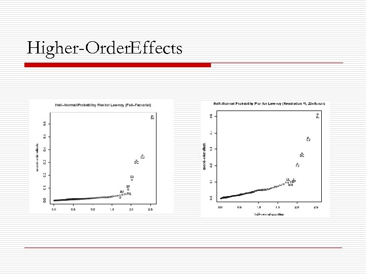
Higher Order. Effects o o Resolution VI design Increased the run size to 2, 048 to capture the second-order effects.

Higher Order. Effects

Higher Order. Effects o o The important interaction effects involve only options that are already considered important by themselves The screening design correctly identifies the 5 most important pairwise interactions at 1/8 th the cost of exhaustive testing.

Thank you