Macroeconomics Class 3 Economic Growth cont

Macroeconomics Class 3: Economic Growth (cont. )

This class: tying lose ends left from Class 2 “globalisation”, externalities and increasing returns to scale Growth under “globalisation” • where accumulation may be funded by foreign savers • The costs and the benefits of globalization (and liberalization) • The concept of an externality • Back to the slow model – evidence on convergence – impediments to convergence – growth with increasing returns to scale 2

Opening the economy to foreign savers In a Solow world: I = S • investment is funded by domestic savings In an open economy, foreign savings are an additional resource That would generate a balance-of-payments (BOP) deficit • but would accelerate convergence Hence, the convergence result is strengthened in an open economy 3

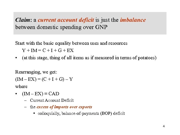Claim: a current account deficit is just the imbalance between domestic spending over GNP Start with the basic equality between uses and resources Y + IM = C + I + G + EX • (at this stage, thing of all items as if measured in terms of potatoes) Rearranging, we get: (IM – EX) = (C + I + G) – Y where • (IM – EX) ≡ CAD – Current Account Deficit – the excess of imports over exports • colloquially, balance-of-payments (BOP) deficit 4

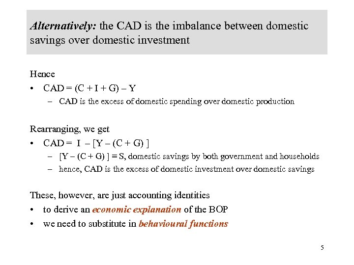Alternatively: the CAD is the imbalance between domestic savings over domestic investment Hence • CAD = (C + I + G) – Y – CAD is the excess of domestic spending over domestic production Rearranging, we get • CAD = I – [Y – (C + G) ] ≡ S, domestic savings by both government and households – hence, CAD is the excess of domestic investment over domestic savings These, however, are just accounting identities • to derive an economic explanation of the BOP • we need to substitute in behavioural functions 5

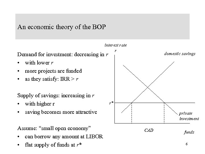An economic theory of the BOP interest rate r domestic savings Demand for investment: decreasing in r • with lower r • more projects are funded • as they satisfy: IRR > r Supply of savings: increasing in r • with higher r • saving becomes more attractive Assume: “small open economy” • can borrow any amount at LIBOR • flat supply of funds at r* r* private investment CAD funds 6

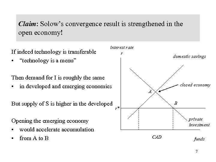Claim: Solow’s convergence result is strengthened in the open economy! If indeed technology is transferable • “technology is a menu” interest rate r Then demand for I is roughly the same • in developed and emerging economies But supply of S is higher in the developed Opening the emerging economy • would accelerate accumulation • from A to B domestic savings closed economy A B r* private investment CAD funds 7

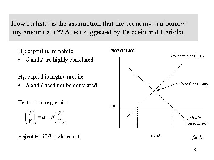How realistic is the assumption that the economy can borrow any amount at r*? A test suggested by Feldsein and Harioka H 0: capital is immobile • S and I are highly correlated interest rate domestic savings H 1: capital is highly mobile • S and I need not be correlated Test: run a regression closed economy r* private investment Reject H 1 if β is close to 1 CAD funds 8

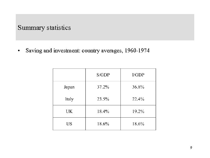Summary statistics • Saving and investment: country averages, 1960 -1974 9

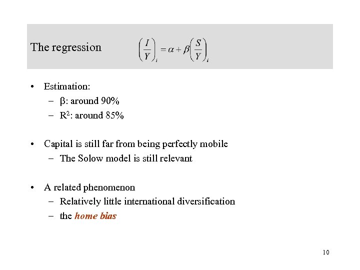The regression • Estimation: – : around 90% – R 2: around 85% • Capital is still far from being perfectly mobile – The Solow model is still relevant • A related phenomenon – Relatively little international diversification – the home bias 10

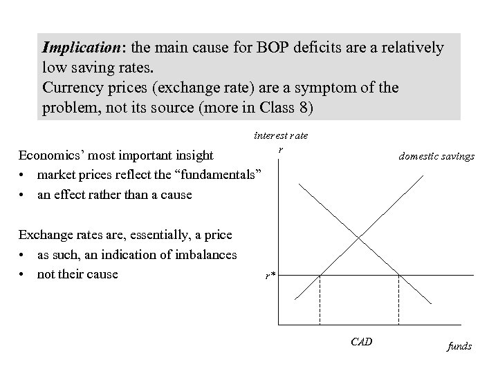Implication: the main cause for BOP deficits are a relatively low saving rates. Currency prices (exchange rate) are a symptom of the problem, not its source (more in Class 8) interest rate r Economics’ most important insight • market prices reflect the “fundamentals” • an effect rather than a cause Exchange rates are, essentially, a price • as such, an indication of imbalances • not their cause domestic savings r* CAD funds 11

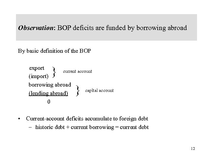Observation: BOP deficits are funded by borrowing abroad By basic definition of the BOP export current account (import) borrowing abroad capital account (lending abroad) 0 } } • Current-account deficits accumulate to foreign debt – historic debt + current borrowing = current debt 12

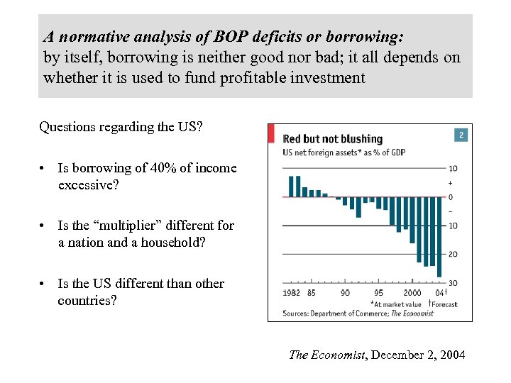A normative analysis of BOP deficits or borrowing: by itself, borrowing is neither good nor bad; it all depends on whether it is used to fund profitable investment Questions regarding the US? • Is borrowing of 40% of income excessive? • Is the “multiplier” different for a nation and a household? • Is the US different than other countries? The Economist, December 2, 2004 13

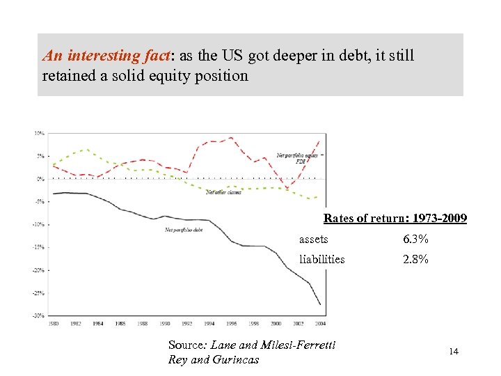An interesting fact: as the US got deeper in debt, it still retained a solid equity position Rates of return: 1973 -2009 assets 6. 3% liabilities 2. 8% Source: Lane and Milesi-Ferretti Rey and Gurincas 14

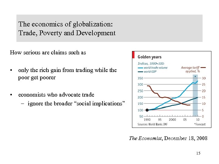The economics of globalization: Trade, Poverty and Development How serious are claims such as • only the rich gain from trading while the poor get poorer • economists who advocate trade – ignore the broader “social implications” The Economist, December 18, 2008 15

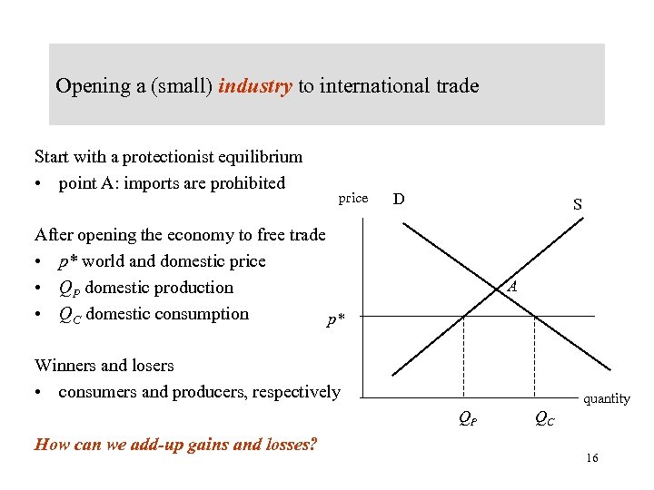Opening a (small) industry to international trade Start with a protectionist equilibrium • point A: imports are prohibited price D S After opening the economy to free trade • p* world and domestic price • QP domestic production • QC domestic consumption p* A Winners and losers • consumers and producers, respectively quantity QP How can we add-up gains and losses? QC 16

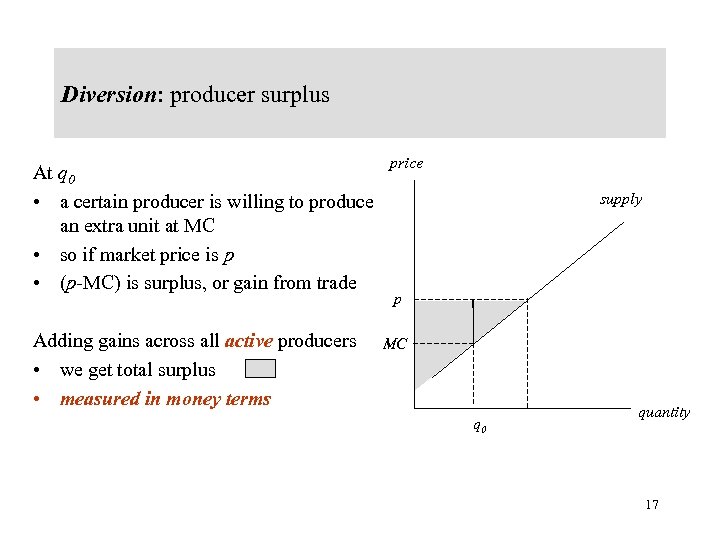Diversion: producer surplus At q 0 • a certain producer is willing to produce an extra unit at MC • so if market price is p • (p-MC) is surplus, or gain from trade Adding gains across all active producers • we get total surplus • measured in money terms price supply p MC q 0 quantity 17

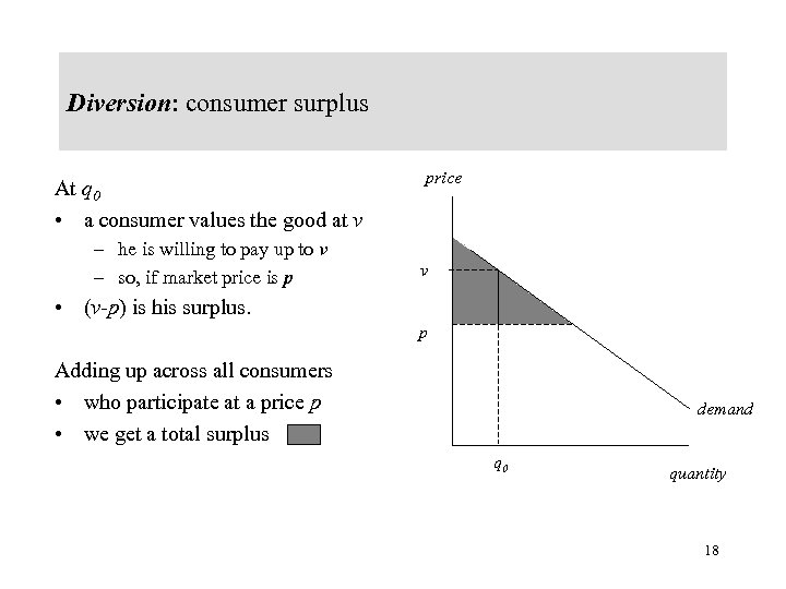Diversion: consumer surplus At q 0 • a consumer values the good at v – he is willing to pay up to v – so, if market price is p price v • (v-p) is his surplus. p Adding up across all consumers • who participate at a price p • we get a total surplus demand q 0 quantity 18

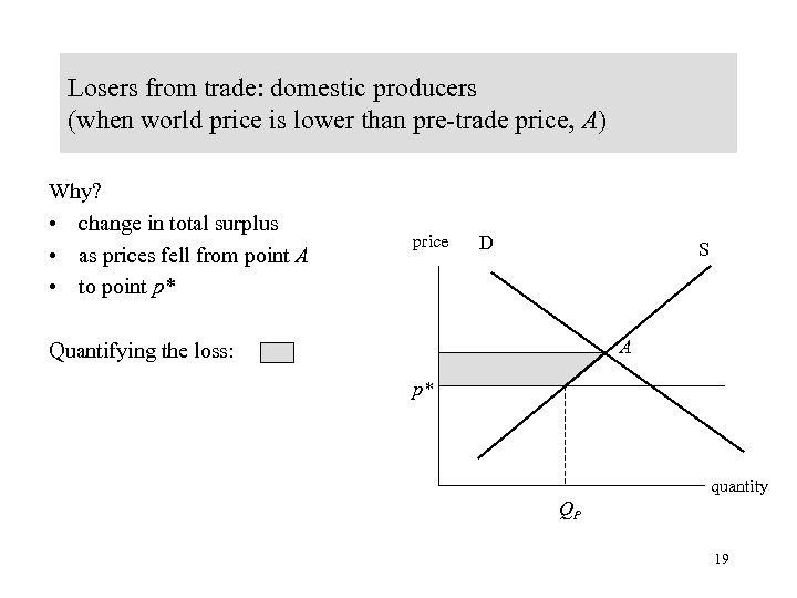Losers from trade: domestic producers (when world price is lower than pre-trade price, A) Why? • change in total surplus • as prices fell from point A • to point p* price D S A Quantifying the loss: p* quantity QP 19

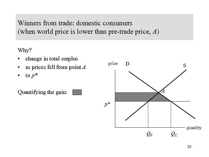Winners from trade: domestic consumers (when world price is lower than pre-trade price, A) Why? • change in total surplus • as prices fell from point A • to p* price D S A Quantifying the gain: p* quantity QP QC 20

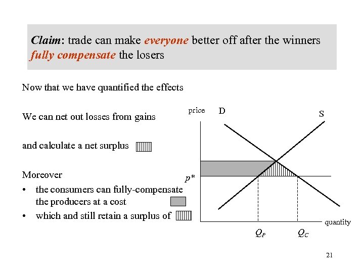Claim: trade can make everyone better off after the winners fully compensate the losers Now that we have quantified the effects We can net out losses from gains price D S and calculate a net surplus Moreover p* • the consumers can fully-compensate the producers at a cost • which and still retain a surplus of quantity QP QC 21

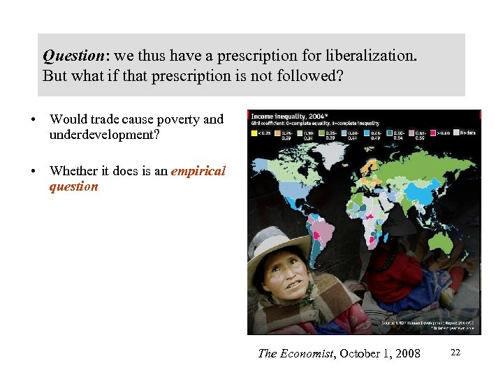Question: we thus have a prescription for liberalization. But what if that prescription is not followed? • Would trade cause poverty and underdevelopment? • Whether it does is an empirical question The Economist, October 1, 2008 22

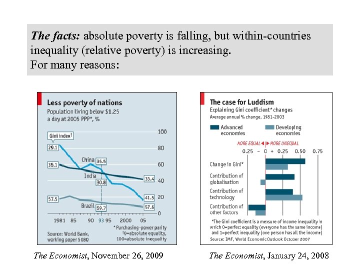The facts: absolute poverty is falling, but within-countries inequality (relative poverty) is increasing. For many reasons: The Economist, November 26, 2009 23 The Economist, January 24, 2008

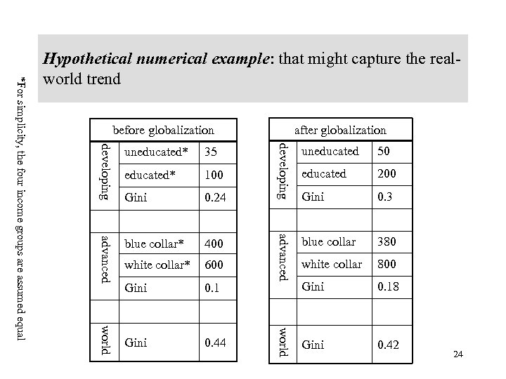after globalization before globalization 100 Gini 0. 24 advanced blue collar* 400 white collar* 600 Gini 0. 1 Gini 0. 44 50 educated 200 Gini 0. 3 blue collar 380 white collar 800 Gini 0. 18 Gini 0. 42 world educated* uneducated advanced 35 developing uneducated* world developing *For simplicity, the four income groups are assumed equal Hypothetical numerical example: that might capture the realworld trend 24

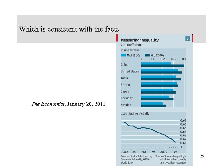Which is consistent with the facts The Economist, January 20, 2011 25

Anecdotal evidence: is trade the source of inequality, or might it be political patronage? Daily Mail, October 8, 2007 Based on a study by Philip Beresford and Bill Rubinstein 26

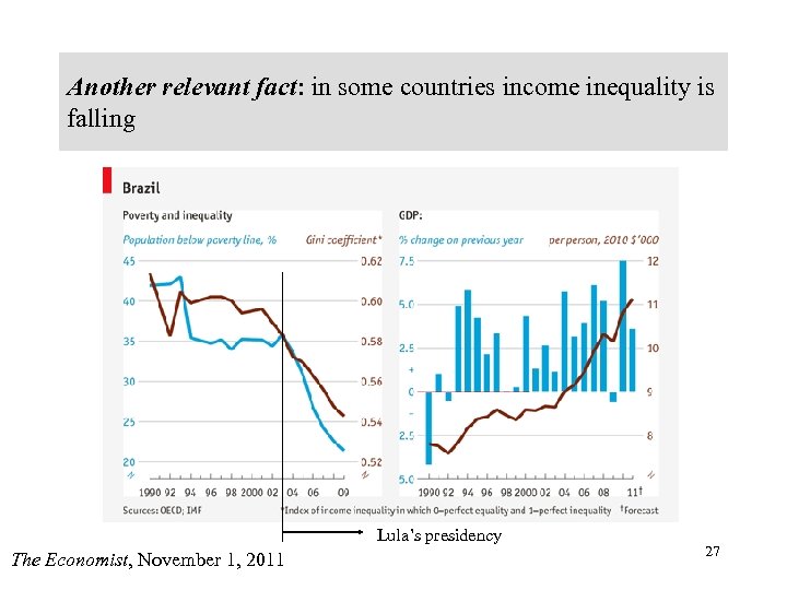Another relevant fact: in some countries income inequality is falling Lula’s presidency The Economist, November 1, 2011 27

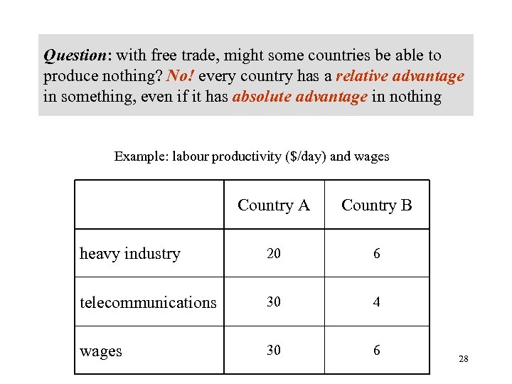Question: with free trade, might some countries be able to produce nothing? No! every country has a relative advantage in something, even if it has absolute advantage in nothing Example: labour productivity ($/day) and wages Country A Country B heavy industry 20 6 telecommunications 30 4 wages 30 6 28

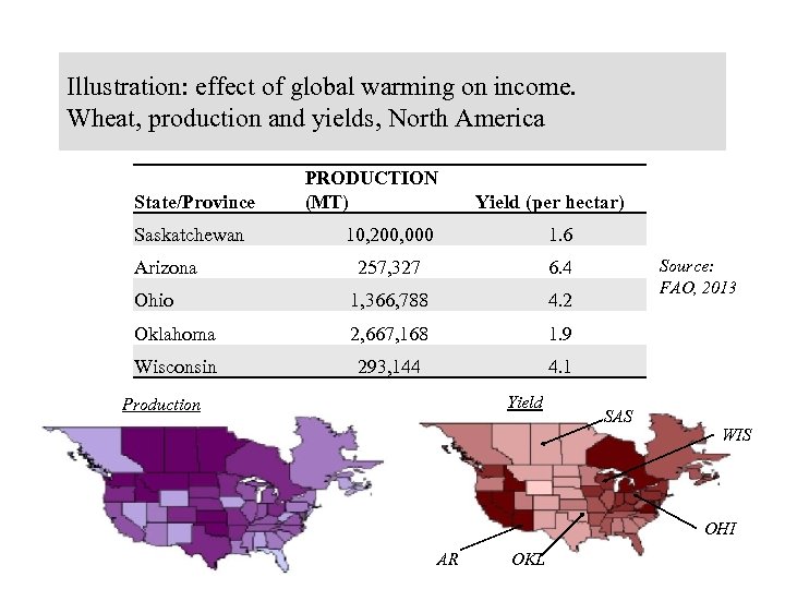Illustration: effect of global warming on income. Wheat, production and yields, North America State/Province Saskatchewan PRODUCTION (MT) Yield (per hectar) 10, 200, 000 1. 6 257, 327 6. 4 Ohio 1, 366, 788 4. 2 Oklahoma 2, 667, 168 1. 9 Wisconsin 293, 144 4. 1 Arizona Yield Production Source: FAO, 2013 SAS WIS OHI AR OKL 29

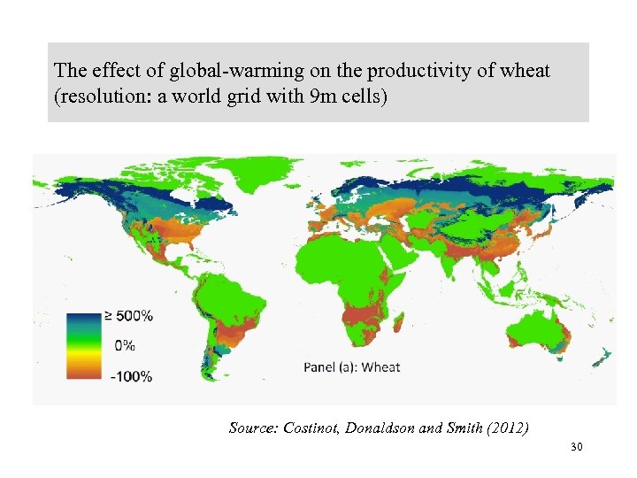The effect of global-warming on the productivity of wheat (resolution: a world grid with 9 m cells) Source: Costinot, Donaldson and Smith (2012) 30

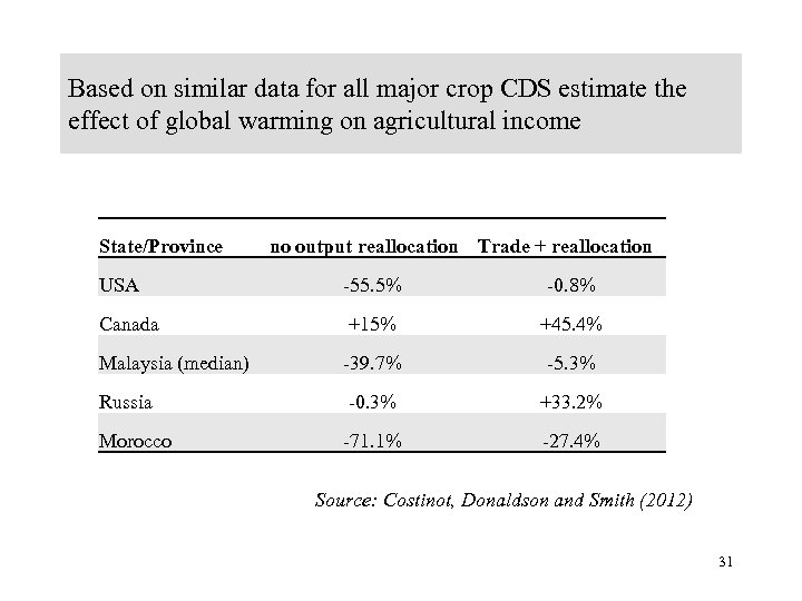Based on similar data for all major crop CDS estimate the effect of global warming on agricultural income State/Province no output reallocation Trade + reallocation USA -55. 5% -0. 8% Canada +15% +45. 4% Malaysia (median) -39. 7% -5. 3% Russia -0. 3% +33. 2% Morocco -71. 1% -27. 4% Source: Costinot, Donaldson and Smith (2012) 31

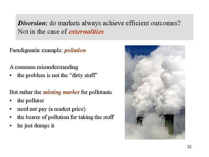Diversion: do markets always achieve efficient outcomes? Not in the case of externalities Paradigmatic example: pollution A common misunderstanding • the problem is not the “dirty stuff” But rather the missing market for pollutants • the polluter • need not pay (a market price) • the bearer of pollution for taking the stuff • he just dumps it 32

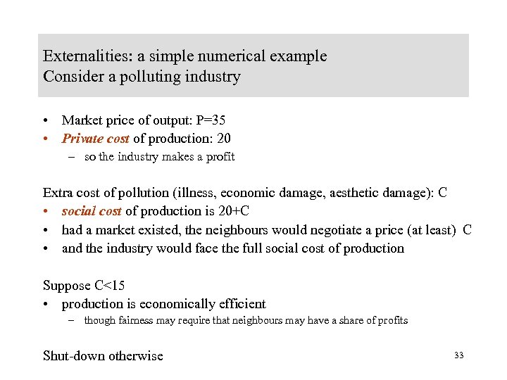Externalities: a simple numerical example Consider a polluting industry • Market price of output: P=35 • Private cost of production: 20 – so the industry makes a profit Extra cost of pollution (illness, economic damage, aesthetic damage): C • social cost of production is 20+C • had a market existed, the neighbours would negotiate a price (at least) C • and the industry would face the full social cost of production Suppose C<15 • production is economically efficient – though fairness may require that neighbours may have a share of profits Shut-down otherwise 33

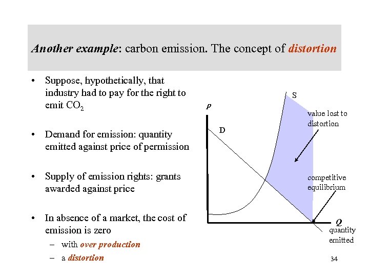Another example: carbon emission. The concept of distortion • Suppose, hypothetically, that industry had to pay for the right to emit CO 2 • Demand for emission: quantity emitted against price of permission • Supply of emission rights: grants awarded against price • In absence of a market, the cost of emission is zero – with over production – a distortion S p D value lost to distortion competitive equilibrium Q quantity emitted 34

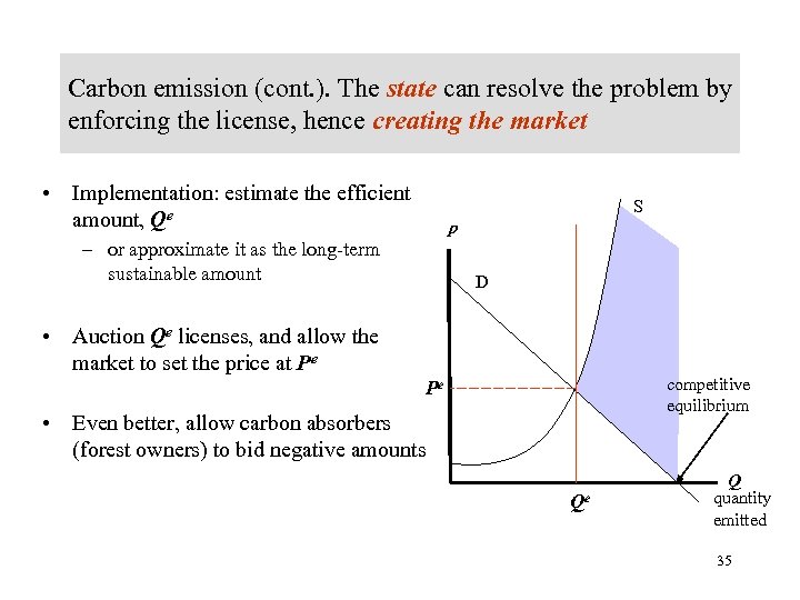Carbon emission (cont. ). The state can resolve the problem by enforcing the license, hence creating the market • Implementation: estimate the efficient amount, Qe S p – or approximate it as the long-term sustainable amount D • Auction Qe licenses, and allow the market to set the price at Pe competitive equilibrium Pe • Even better, allow carbon absorbers (forest owners) to bid negative amounts Qe Q quantity emitted 35

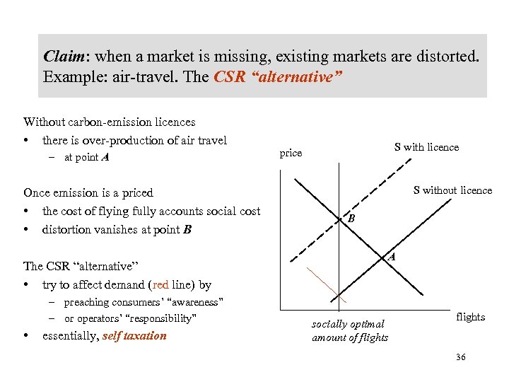Claim: when a market is missing, existing markets are distorted. Example: air-travel. The CSR “alternative” Without carbon-emission licences • there is over-production of air travel – at point A Once emission is a priced • the cost of flying fully accounts social cost • distortion vanishes at point B The CSR “alternative” • try to affect demand (red line) by – preaching consumers’ “awareness” – or operators’ “responsibility” • essentially, self taxation S with licence price S without licence B A socially optimal amount of flights 36

The “old fashioned” approach: some goods (services) have no market; the state should regulate their production Goods that have no market: public goods For example • law and order • protection of property rights • defence • regulating emission In practice, identifying externalities is difficult and contested • for example: education, health, equal opportunities, fairness 37

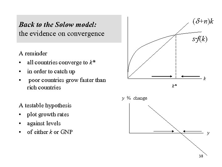( +n)k Back to the Solow model: the evidence on convergence s·f(k) A reminder • all countries converge to k* • in order to catch up • poor countries grow faster than rich countries k k* y % change A testable hypothesis • plot growth rates • against levels • of either k or GNP y 38

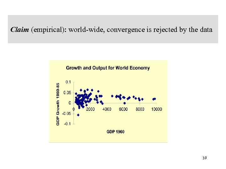Claim (empirical): world-wide, convergence is rejected by the data 39

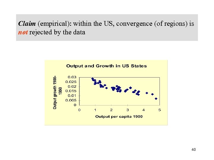Claim (empirical): within the US, convergence (of regions) is not rejected by the data 40

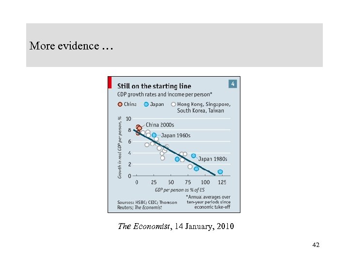
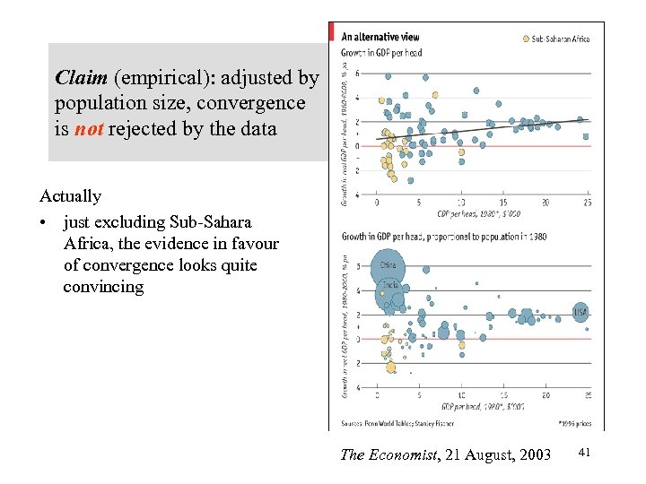Claim (empirical): adjusted by population size, convergence is not rejected by the data Actually • just excluding Sub-Sahara Africa, the evidence in favour of convergence looks quite convincing The Economist, 21 August, 2003 41

More evidence … The Economist, 14 January, 2010 42

So why are some countries left behind? Non technological factors: corruption Source: Transparency International, 2012 43

Individual countries Country Rank Score Denmark 1 90 Singapore 5 87 Hong Kong 14 77 UK 17 74 South Africa 69 43 Brazil 69 43 Italy 72 42 Greece 94 36 India 94 36 Pakistan 139 27 Somalia 174 8 44

More precise measurement: Ease of doing business The Economist, September 15, 2005 45

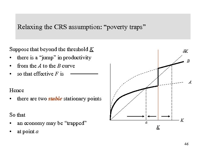Relaxing the CRS assumption: “poverty traps” Suppose that beyond the threshold K • there is a “jump” in productivity • from the A to the B curve • so that effective F is K B A Hence • there are two stable stationary points So that • an economy may be “trapped” • at point a K 46

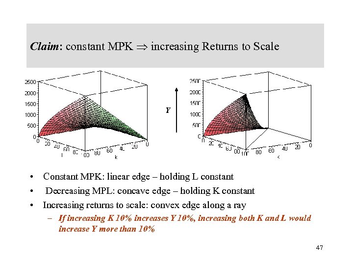Claim: constant MPK increasing Returns to Scale Y • Constant MPK: linear edge – holding L constant • Decreasing MPL: concave edge – holding K constant • Increasing returns to scale: convex edge along a ray – If increasing K 10% increases Y 10%, increasing both K and L would increase Y more than 10% 47

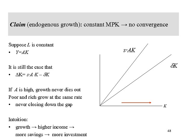Claim (endogenous growth): constant MPK → no convergence Suppose L is constant • Y=AK s·AK K It is still the case that • K= s·A K – K If A is high, growth never dies out Poor and rich grow at the same rate • never closing down the gap Intuition: • growth → higher income → more savings → more investment K 48

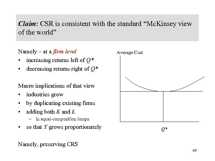Claim: CSR is consistent with the standard “Mc. Kinsey view of the world” Namely – at a firm level • increasing returns left of Q* • decreasing returns right of Q* Average Cost Macro implications of that view • industries grow • by duplicating existing firms • adding both K and L – in equal-composition lumps • so that Y grows proportionately Q* Namely, preserving CRS 49

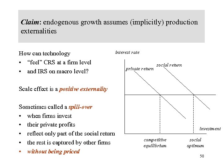Claim: endogenous growth assumes (implicitly) production externalities How can technology • “feel” CRS at a firm level • and IRS on macro level? interest rate private return social return Scale effect is a positive externality Sometimes called a spill-over • when firms invest • their private profits • reflect only part of the social return • the rest is captured by other firms • without being priced investment competitive equilibrium social optimum 50

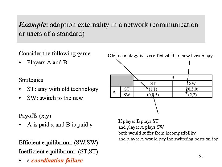Example: adoption externality in a network (communication or users of a standard) Consider the following game • Players A and B Old technology is less efficient than new technology Strategies • ST: stay with old technology • SW: switch to the new Payoffs (x, y) • A is paid x and B is paid y Efficient equilibrium: (SW, SW) Inefficient equilibrium: (ST, ST) • a coordination failure If player B plays ST and player A plays SW both would suffer from incompatibility and player A would pay the switching costs on top 51

Real world example of network externalities: QWERTY is the standard for key-boards (in English) • inherited from the type-writer Standards are paradigmatic examples of network externalities • the value of adopting a standard • is a function of others adopting the same standard 52

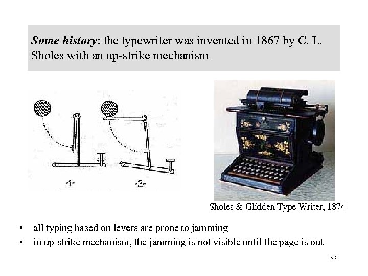Some history: the typewriter was invented in 1867 by C. L. Sholes with an up-strike mechanism Sholes & Glidden Type Writer, 1874 • all typing based on levers are prone to jamming • in up-strike mechanism, the jamming is not visible until the page is out 53

Claim (by Paul David): the QWERTY standard is inefficient Evidence for the inefficiency • QWERTY was invented with the deliberate intention of slowing down the speed of typing (in order to avoid jamming) • a more efficient arrangement exist – Dvorak Simplified Keyboard, DSK – where keys for high-frequency letters are concentrated • the US Navy (1940) has estimated that retraining a secretary would pay back within 10 days • some Apple models offered a button to switch standard – with an increased typing speed of 20 -40% 54

… and its survival is an “historic accident” Still, the more efficient technology was never adopted Interpretation • the industry is stuck in the (ST, ST) equilibrium Each player expects that the others are conservative, and would play ST • hence, switching implies bearing a cost • and becoming incompatible with other’s typewriters Conclusion • spill-overs probably exist, but it is doubtful whether they are so pervasive so as to seriously undermine CRS on a macro scale 55

Implication: with positive externalities, competitive equilibrium will be economically inefficient. To restore efficiency, the state has to implement industrial policy While negative externalities lead to over production • to be resolved by way of taxation Positive externalities lead to under production • to be resolved by way of investment subsidies • so that investing companies would internalize the full economic value that they generate Such policies widely used in the 1950 s in South America • never worked in practice 56

Summary (my own view) • While examples of the sort of QWERTY are convincing enough • There is no evidence that their quantitative effect, on a macro level, is strong enough to make the Solow model irrelevant • Better view the process of accumulation is critical to economic growth – and treat technological innovations as an exogenous process • At the same time, the role of the state in providing infrastructure, law and order, protection of property rights etc. – is absolutely essential 57