Macroeconomic Experiments my take Charles Noussair Tilburg University

Macroeconomic Experiments (my take) Charles Noussair Tilburg University June 9, 2011

Outline of this lecture • Four illustrations (examples of topics that one could study): – – Growth Models Multiple Equilibria and Poverty Traps DSGE economies International Economies • All four have features that: – Stick close to an existing theoretical model • Easier to communicate • Have hypotheses and benchmark predictions – Have a specific research question as a focus

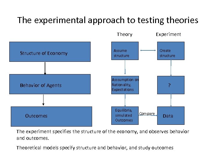
The experimental approach to testing theories Theory Structure of Economy Behavior of Agents Outcomes Experiment Assume structure Create structure Asssumption on Rationality, Expectations Equilibria, simulated Outcomes Compare ? Data The experiment specifies the structure of the economy, and observes behavior and outcomes. Theoretical models specify structure and behavior, and study outcomes

Application I: Dynamic Economies; Testing Growth Models • Reference (Lei and Noussair, 2002) • Most experiments consist of repetition of a stationary environment with no dynamic link between periods. • Macroeconomic models directly focus on intertemporal linkages between variables, such as between savings and future consumption. • This experiment illustrates one way intertemporal design issues can be approached.

Theoretical Model: The Ramsey/Cass/Koopmans Model of Optimal Growth • A representative consumer in the economy has a lifetime utility given by • ρ is the discount rate, Ct is the quantity of consumption at time t, and U(Ct) is the utility of consumption. The economy faces the resource constraint: • δ is the depreciation rate, Kt is the economy’s aggregate capital stock at the beginning of period t, and A is an efficiency parameter on the production technology. Under the assumption that the production function is concave, the principal predictin of the model is that Ct and Kt converge asymptotically to optimal steady state levels. The optimal steady state given by the solution to: • • C* = F(K*) – δK* K* = ρ + δ

• The behavior of this economy (in theory) can be interpreted as: – The solution to an optimization problem of a benevolent social planner – The rational expectations equilibrium of a decentralized market economy • The experiment considers two issues: 1) Do economies with this structure convergence to the optimal steady state? 2) How important is the institutional structure to obtain convergence to the optimal steady state?

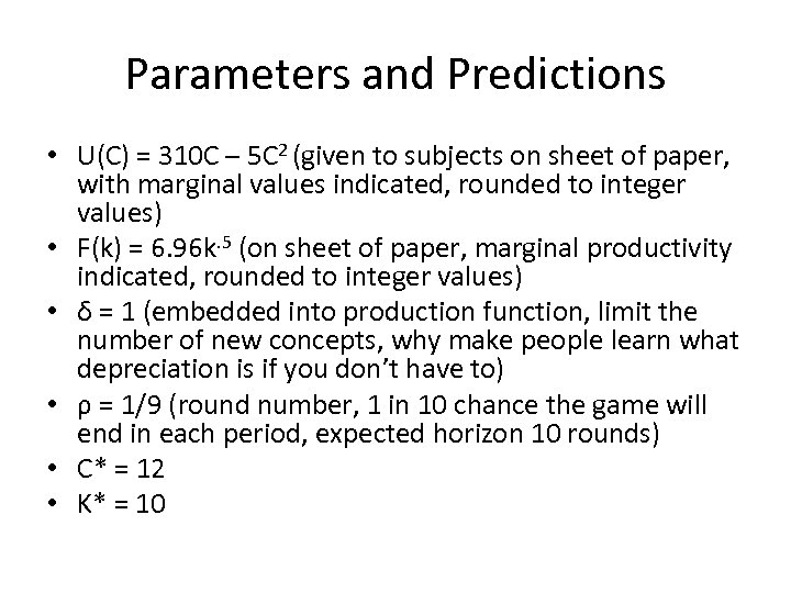
Parameters and Predictions • U(C) = 310 C – 5 C 2 (given to subjects on sheet of paper, with marginal values indicated, rounded to integer values) • F(k) = 6. 96 k. 5 (on sheet of paper, marginal productivity indicated, rounded to integer values) • δ = 1 (embedded into production function, limit the number of new concepts, why make people learn what depreciation is if you don’t have to) • ρ = 1/9 (round number, 1 in 10 chance the game will end in each period, expected horizon 10 rounds) • C* = 12 • K* = 10

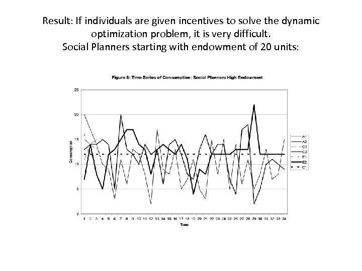
Result: If individuals are given incentives to solve the dynamic optimization problem, it is very difficult. Social Planners starting with endowment of 20 units:

Suppose a team of five people is making the decision instead. They still have a lot of trouble

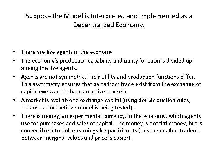
Suppose the Model is Interpreted and Implemented as a Decentralized Economy. • There are five agents in the economy • The economy’s production capability and utility function is divided up among the five agents. • Agents are not symmetric. Their utility and production functions differ. This asymmetry ensures that gains from trade exist from the exchange of capital (we want to have an active market). • A market is available to exchange capital (using double auction rules, because a competitive model is being tested). • There is money, an experimental currency, in the economy, which agents use for purchases and sales of capital. The money is not fiat money, but is convertible into dollar earnings for participants (this means that tradeoff between marginal values and price is easier).

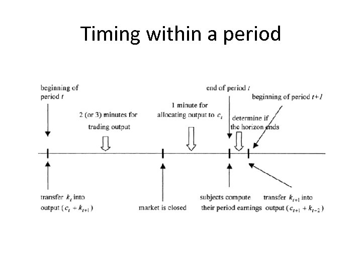
Timing within a period t • At the beginning of period t, production occurs mapping kt into output (ct + kt+1) • A double auction market for output is open for two minutes in which they can exchange output. • Agents have one minute to allocate any portion of their output to consumption ct • At the beginning of period t+1, production occurs mapping kt+1 into output (ct+1 + kt+2). • A common issue that arises in macroexperiments is the lack of explicit timing in macroeconomic models.

Timing within a period

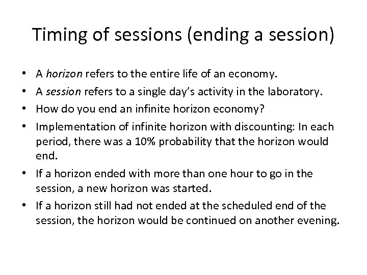
Timing of sessions (ending a session) A horizon refers to the entire life of an economy. A session refers to a single day’s activity in the laboratory. How do you end an infinite horizon economy? Implementation of infinite horizon with discounting: In each period, there was a 10% probability that the horizon would end. • If a horizon ended with more than one hour to go in the session, a new horizon was started. • If a horizon still had not ended at the scheduled end of the session, the horizon would be continued on another evening. • •

• Subjects would have the option of continuing in their roles in the continued session. • If they chose not to continue, a substitute would be recruited to take her place. The original subject would also receive the money earned by the substitute.

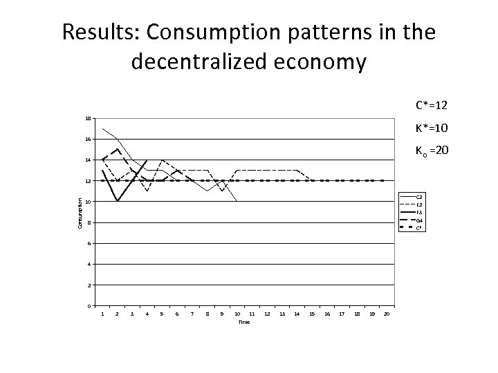
Results: Consumption patterns in the decentralized economy C*=12 18 K*=10 16 Ko =20 14 Consumption 12 C 2 E 2 F 3 G 4 C* 10 8 6 4 2 0 1 2 3 4 5 6 7 8 9 10 11 Time 12 13 14 15 16 17 18 19 20

Summary of results • When individuals are presented with the social planner’s optimization problem, the economies perform poorly. • Institutions have an impact on the level and variance of output and on welfare • The decentralized market economy converges to the optimal steady state. – The key appears to be the existence of an endogenous market price for capital revealing it’s scarcity.

Application II: Multiple Equilibria in Dynamic Economies (source is Capra et al. , 2009) • The existence of multiple equilibria can (theoretically) explain differences in income between countries, even if they have identical institutions (Rosenstein-Rodan, 1943; Murphy et al. , 1989; Azariadis, 1990; Galor and Zeira, 1993; Ray, 2003). • Unfortunate countries may find themselves in an inferior equilibrium, a “poverty trap”. • Institutions may play a role if multiple equilibria exist. Some institutions may facilitate successful coordination on better equilibria.

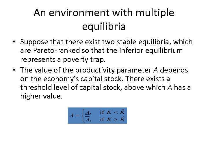
An environment with multiple equilibria • Suppose that there exist two stable equilibria, which are Pareto-ranked so that the inferior equilibrium represents a poverty trap. • The value of the productivity parameter A depends on the economy’s capital stock. There exists a threshold level of capital stock, above which A has a higher value.

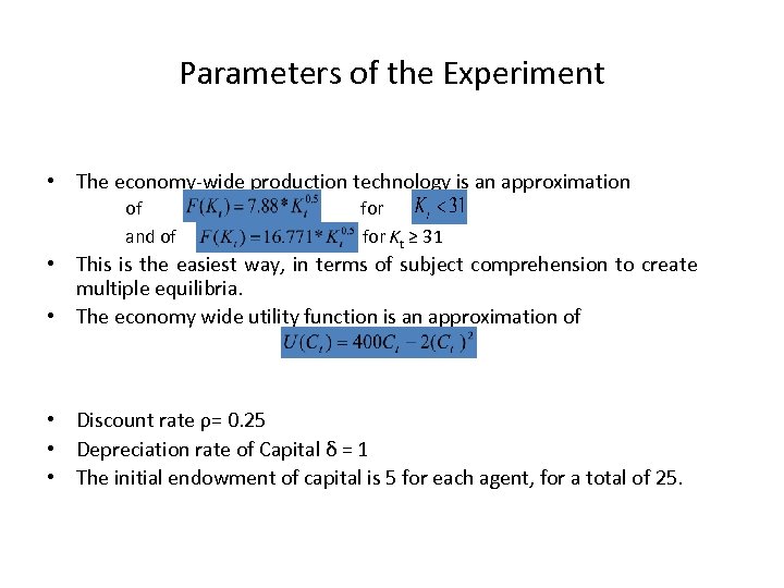
Parameters of the Experiment • The economy-wide production technology is an approximation of for and of for Kt ≥ 31 • This is the easiest way, in terms of subject comprehension to create multiple equilibria. • The economy wide utility function is an approximation of • Discount rate ρ= 0. 25 • Depreciation rate of Capital δ = 1 • The initial endowment of capital is 5 for each agent, for a total of 25.

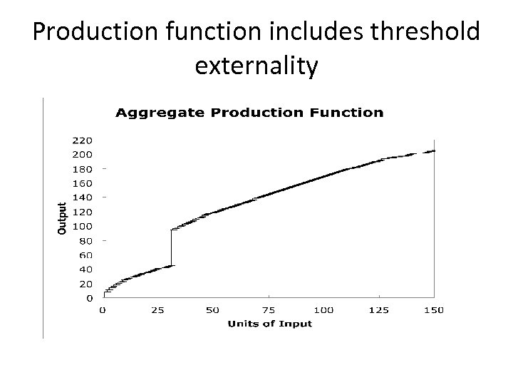
Production function includes threshold externality

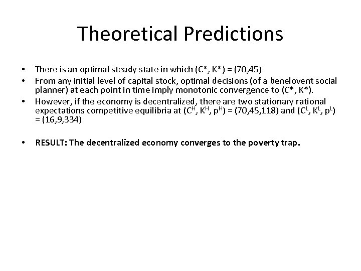
Theoretical Predictions • • • • There is an optimal steady state in which (C*, K*) = (70, 45) From any initial level of capital stock, optimal decisions (of a benelovent social planner) at each point in time imply monotonic convergence to (C*, K*). However, if the economy is decentralized, there are two stationary rational expectations competitive equilibria at (CH, KH, p. H) = (70, 45, 118) and (CL, KL, p. L) = (16, 9, 334) RESULT: The decentralized economy converges to the poverty trap.

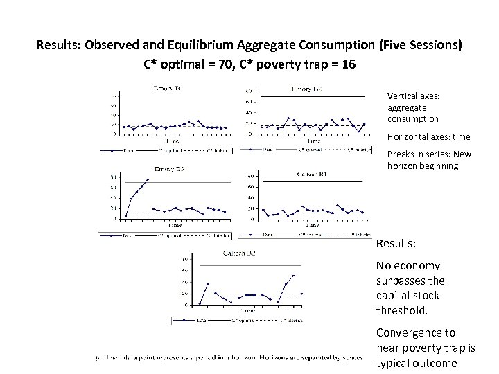
Results: Observed and Equilibrium Aggregate Consumption (Five Sessions) C* optimal = 70, C* poverty trap = 16 Vertical axes: aggregate consumption Horizontal axes: time Breaks in series: New horizon beginning Results: No economy surpasses the capital stock threshold. Convergence to near poverty trap is typical outcome

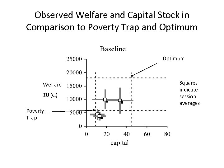
Observed Welfare and Capital Stock in Comparison to Poverty Trap and Optimum Welfare ΣUi(ct) Poverty Trap Squares indicate session averages

Research question: What institutions can improve on these outcomes? • This parametric structure provides a challenging environment for additional institutions to avoid/exit the poverty trap. • We consider whether two institutions, communication and voting, alone or together, can improve outcomes in this economy. – Voting is a stylized version of “democracy” and – Communication is a stylized version of “freedom of expression (free press)”,

The Communication treatment – Identical to the baseline treatment, except that before the market opened, subjects were allowed to communicate with each other. – Each agent’s screen displayed a chat-room, which they could use to send and receive messages in real time. – Communication was unrestricted and all agents could observe all messages.

Observed and Equilibrium Aggregate Consumption, Communication Treatment; C* optimal = 70, C* inferior = 16 Results: Individual sessions converge to near one of the equilibria. Vertical axes: aggregate consumption Horizontal axes: time Breaks in series: New horizon beginning However, which equilibrium it converges to varies between sessions. Example of how institutional structure affects mean and variance of income.

The Voting treatment – – – Identical to the baseline treatment except that consumption and investment decisions were determined in the following manner: Two agents were randomly chosen in each period to make proposals on how much each agent in the economy should consume. Before submitting proposals, proposers received information indicating the current stock of capital held by each agent. Proposals were followed by majority voting. All agents were required to vote in favor of exactly one of the two proposals. The proposal that gained at least 3 (of the 5 total) votes became binding. Each agent consumed the quantity of output specified under the winning proposal, and began next period with the amount of capital allotted to her under the winning proposal.

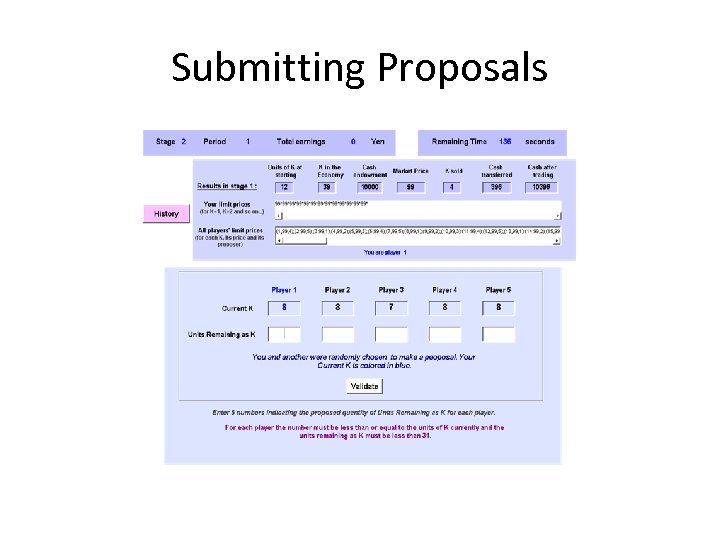
Submitting Proposals

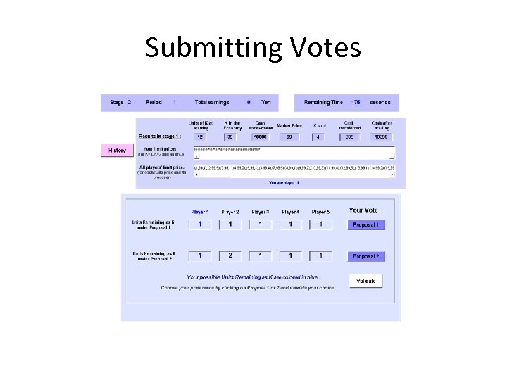
Submitting Votes

Observed and Equilibrium Aggregate Consumption, Voting Treatment C* optimal = 70, C* inferior = 16 Results: Vertical axis: aggregate consumption Horizontal axis: time Breaks in series: New horizon beginning -In most sessions, economy escapes poverty trap - High variance from one period to the next within sessions. - Convergence toward equilibrium typically does not occur

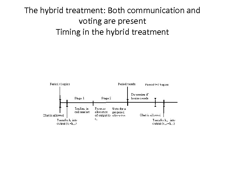
The hybrid treatment: Both communication and voting are present Timing in the hybrid treatment

Observed and Equilibrium Aggregate Consumption, Hybrid Treatment; C* optimal = 70, C* inferior = 16 Vertical axis: aggregate consumption Horizontal axis: time Breaks in series: New horizon beginning Result; The addition of voting and communication allows the economy to escape poverty trap in all sessions.

Results • Baseline: The economies of the baseline treatment converge to near the poverty trap. Does not escape poverty trap in any session. • Communciation: The economies of the communication treatment converges to close to one of the stationary equilibria. However, the one it converges toward varies between sessions. Probability of avoiding the poverty trap greater than under baseline. • Voting: The voting treatment exhibits variable behavior from one period to the next. Probability of avoiding the poverty trap greater than under baseline. • Hybrid: Also shows variable behavior from one period to the next. Escapes the poverty trap in all sessions.

Application III: DSGE models • Construct an experimental New Keynesian DSGE macroeconomy, populated with human agents. • Three types of (infinitely lived) agents – Consumers: supply labor, purchase (3) products, and save for the future – Producers: purchase labor, produce one of the (3) products, sell output – Central bank: sets interest rates • Preferences and productivity subject to shocks

Producer incentives • Maximize profit: Пit = pityit – wt. Lit yit = At. Lit At = A 0 + γAt-1 + δεt Where Пit = profit of firm i in period t pit = price of good i in period t yit = production of good i in t wt = wage in t Lit = labor bought by i in t At = productivity parameter in t εt = productivity shock in t γ = 0. 8, δ = 0. 2, A 0 = 0. 7

Consumer incentives • • • Payoff in period t of consumer j = βt[Ujt(Cjt) – Dj(Ljt)] Ujt(Cjt)=∑ihijt[cijt(1 -σ)/(1 - σ)] hijt = μij + τhijt-1 + δεjt D(Ljt) = d*Ljt 1+η/ (1+η) Where Cjt= consumption at time t of consumer j Ljt = labor supplied at t Dj(Ljt) = disutility to j of labor he supplies at t cijt = consumption of good i by consumer j at t ε jt = preference shock for consumer j in period t β =. 99, μij = 120, τ = 0. 8, d = 15, η = 2, n = 3.

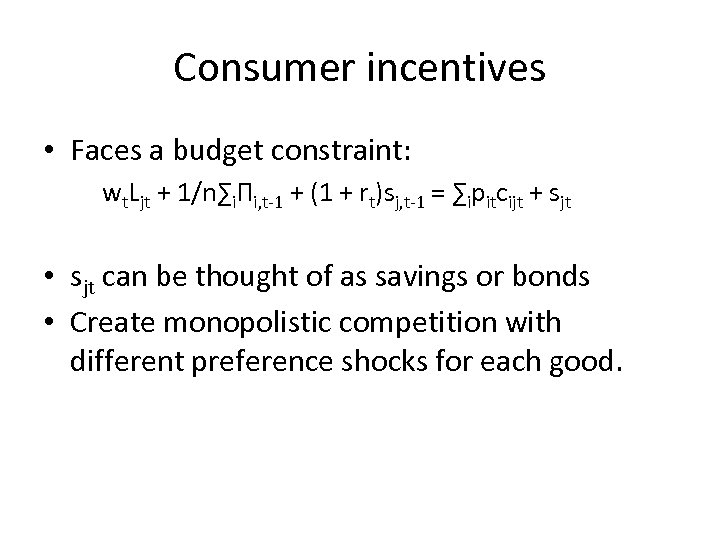
Consumer incentives • Faces a budget constraint: wt. Ljt + 1/n∑iΠi, t-1 + (1 + rt)sj, t-1 = ∑ipitcijt + sjt • sjt can be thought of as savings or bonds • Create monopolistic competition with different preference shocks for each good.

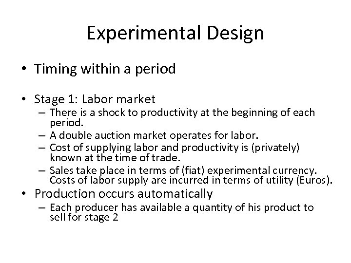
Experimental Design • Timing within a period • Stage 1: Labor market – There is a shock to productivity at the beginning of each period. – A double auction market operates for labor. – Cost of supplying labor and productivity is (privately) known at the time of trade. – Sales take place in terms of (fiat) experimental currency. Costs of labor supply are incurred in terms of utility (Euros). • Production occurs automatically – Each producer has available a quantity of his product to sell for stage 2

Labor market: Consumer

Labor Market: Producer

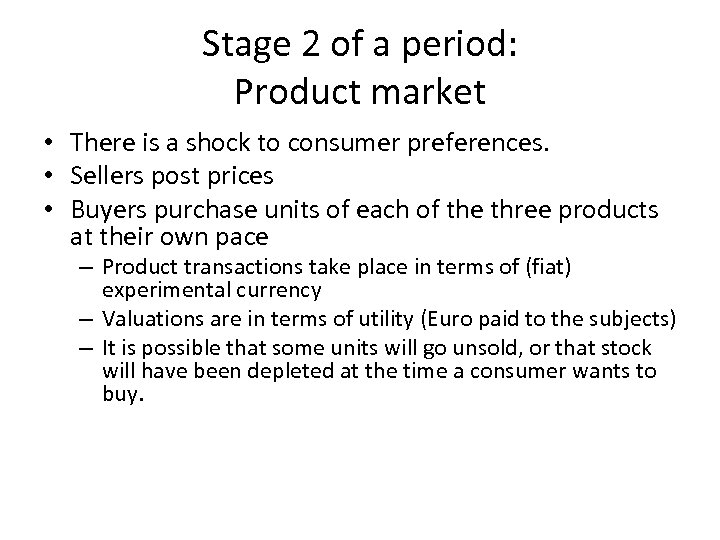
Stage 2 of a period: Product market • There is a shock to consumer preferences. • Sellers post prices • Buyers purchase units of each of the three products at their own pace – Product transactions take place in terms of (fiat) experimental currency – Valuations are in terms of utility (Euro paid to the subjects) – It is possible that some units will go unsold, or that stock will have been depleted at the time a consumer wants to buy.

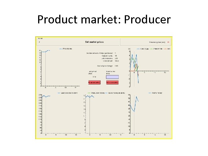
Product market: Producer

Product Market: Consumer

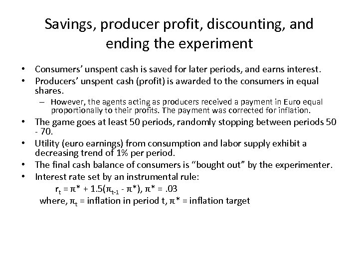
Savings, producer profit, discounting, and ending the experiment • Consumers’ unspent cash is saved for later periods, and earns interest. • Producers’ unspent cash (profit) is awarded to the consumers in equal shares. – However, the agents acting as producers received a payment in Euro equal proportionally to their profits. The payment was corrected for inflation. • The game goes at least 50 periods, randomly stopping between periods 50 - 70. • Utility (euro earnings) from consumption and labor supply exhibit a decreasing trend of 1% period. • The final cash balance of consumers is “bought out” by the experimenter. • Interest rate set by an instrumental rule: rt = π* + 1. 5(πt-1 - π*), π* =. 03 where, πt = inflation in period t, π* = inflation target

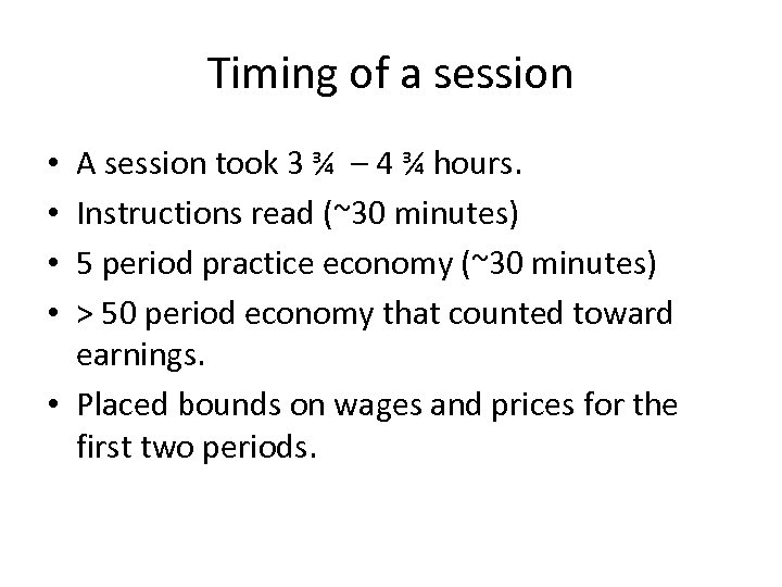
Timing of a session A session took 3 ¾ – 4 ¾ hours. Instructions read (~30 minutes) 5 period practice economy (~30 minutes) > 50 period economy that counted toward earnings. • Placed bounds on wages and prices for the first two periods. • •

The treatments • (1) Baseline – The conditions described above • (2) Human Central Banker: In each period, three agents each chose an interest rate. The group’s decision (and thus the rate in effect) was the median of the three choices. The agents had an incentive to minimize the loss function Losst = (πt – π*)2 Central bankers were paid an amount equal to max{0, a – b*Loss}

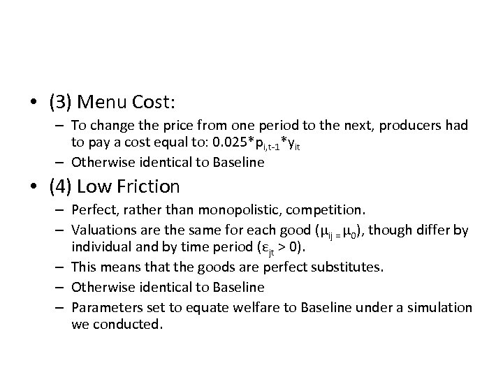
• (3) Menu Cost: – To change the price from one period to the next, producers had to pay a cost equal to: 0. 025*pi, t-1*yit – Otherwise identical to Baseline • (4) Low Friction – Perfect, rather than monopolistic, competition. – Valuations are the same for each good (μij = μ 0), though differ by individual and by time period (εjt > 0). – This means that the goods are perfect substitutes. – Otherwise identical to Baseline – Parameters set to equate welfare to Baseline under a simulation we conducted.

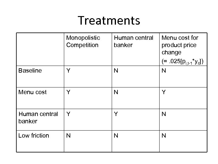
Treatments Monopolistic Competition Human central banker Menu cost for product price change (=. 025[pi, t-1*yit]) Baseline Y N N Menu cost Y N Y Human central banker Y Y N Low friction N N N

Procedures • 16 sessions, four under each treatment • 3 producers and 3 consumers in each session • In the Human Central Banker treatment, there were also three central bankers. • Subjects were undergraduates at Tilburg University • Experiments conducted in English • Average earnings = 43. 99 euro

Hypothesis • Persistence of shocks (effect beyond the current period): – Treatment differences – In treatments Baseline, Human Central Banker, and Low Friction no persistence, in treatment Menu Cost, shocks are persistent (both Menu Cost and market power are needed for persistence in New Keynesian DSGE model). • Empirical stylized fact is that a shock to interest rates, output, or inflation, has persistent effects on itself and on some of the other two variables. • Also can compare between treatments – GDP, inflation, welfare, employment, etc…

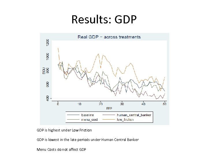
Results: GDP is highest under Low Friction GDP is lowest in the late periods under Human Central Banker Menu Costs do not affect GDP

Results: Inflation -20 Inflation rate 0 20 40 Inflation - across treatments 0 10 20 HCB menu_cost ppp 30 40 50 baseline low_friction Inflation rate is similar on average in all four treatments, including Human Central Bankers Volatility is lowest under Menu costs Volatility is highest under Human Central Banker

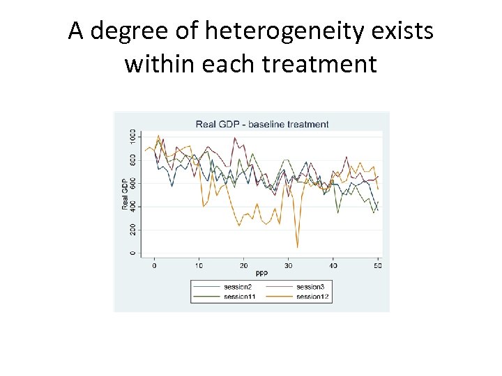
A degree of heterogeneity exists within each treatment

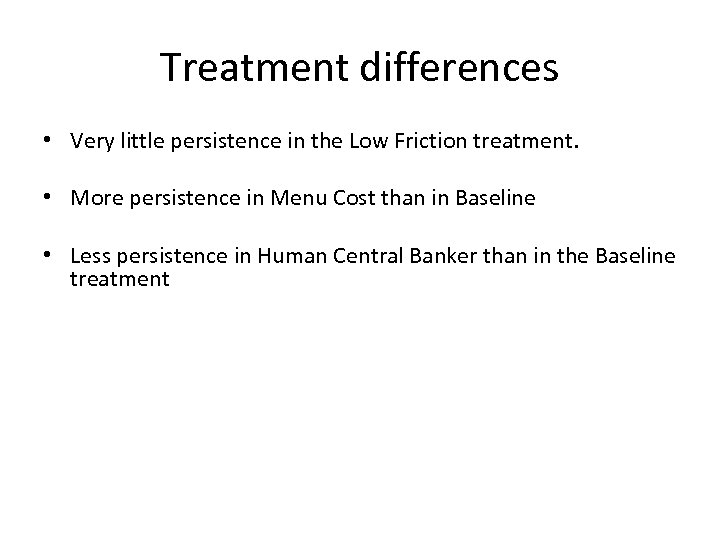
Treatment differences • Very little persistence in the Low Friction treatment. • More persistence in Menu Cost than in Baseline • Less persistence in Human Central Banker than in the Baseline treatment

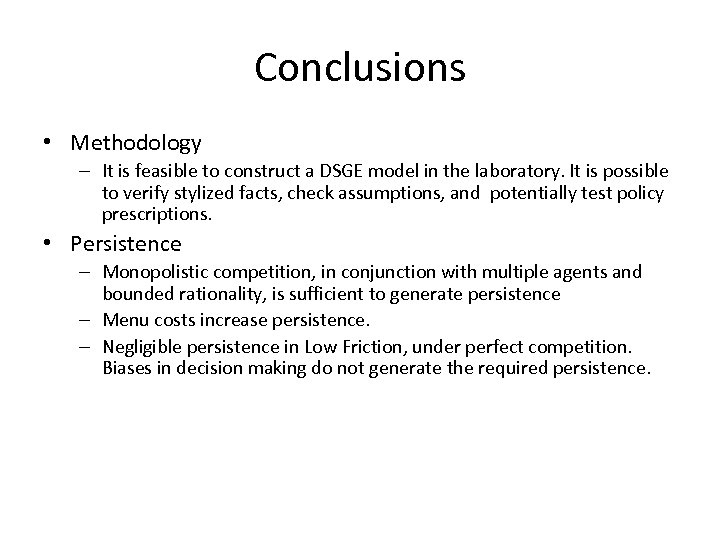
Conclusions • Methodology – It is feasible to construct a DSGE model in the laboratory. It is possible to verify stylized facts, check assumptions, and potentially test policy prescriptions. • Persistence – Monopolistic competition, in conjunction with multiple agents and bounded rationality, is sufficient to generate persistence – Menu costs increase persistence. – Negligible persistence in Low Friction, under perfect competition. Biases in decision making do not generate the required persistence.

Application IV: Multiple Market “International” Economy (Noussair et al. , 2007). • • • Consider a larger scale and more complex economy. 60 subjects divided into three countries of population 20. Trade in each country takes place in terms of its own currency. There are two inputs, V and W residing in each country. There are three outputs X, Y, and Z, all of which can be produced in all three countries from inputs V and W from the same country. Multiple inputs are required to produce each output. Production is Cobb. Douglas f(v, w) = Av. 25 w. 25, with A equaling either 2 or 4. 21 markets: 6 input, 9 output, and 6 currency markets. The research question: Can an economy this complex converge to its competitive equilibrium? Note: Existence theorem for CE does not apply when demand is discrete and there are multiple markets. To parameterize, specify prices and then fit demand supply curves and production functions.

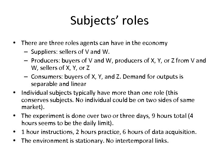
Subjects’ roles • There are three roles agents can have in the economy – Suppliers: sellers of V and W. – Producers: buyers of V and W, producers of X, Y, or Z from V and W, sellers of X, Y, or Z – Consumers: buyers of X, Y, and Z. Demand for outputs is separable and linear • Individual subjects typically have more than one role (this conserves subjects. No individual could be on two sides of same market). • The experiment is done over two or three days, 9 hours total (4 hours seems to be the daily limit). • 1 hour instructions, 2 hours practice, 6 hours of data acquisition. • The environment is stationary. No intertemporal links.

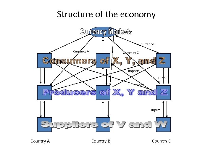
Structure of the economy Currency C Currency A Currency C Imports Exports Outpu t Inputs Country A Country B Country C

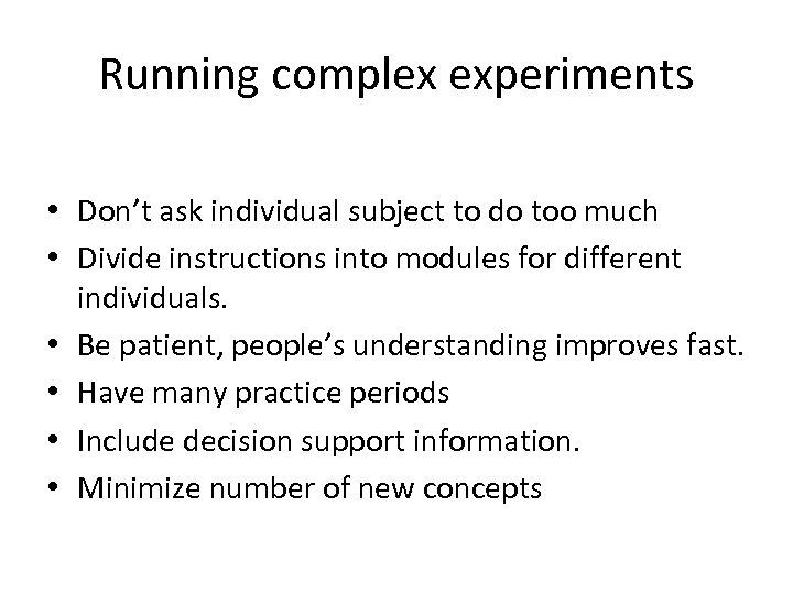
Running complex experiments • Don’t ask individual subject to do too much • Divide instructions into modules for different individuals. • Be patient, people’s understanding improves fast. • Have many practice periods • Include decision support information. • Minimize number of new concepts

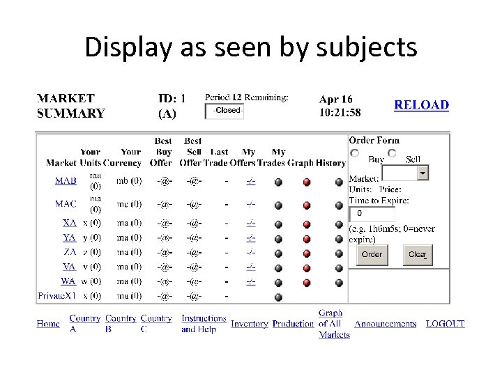
Display as seen by subjects

Production Screen

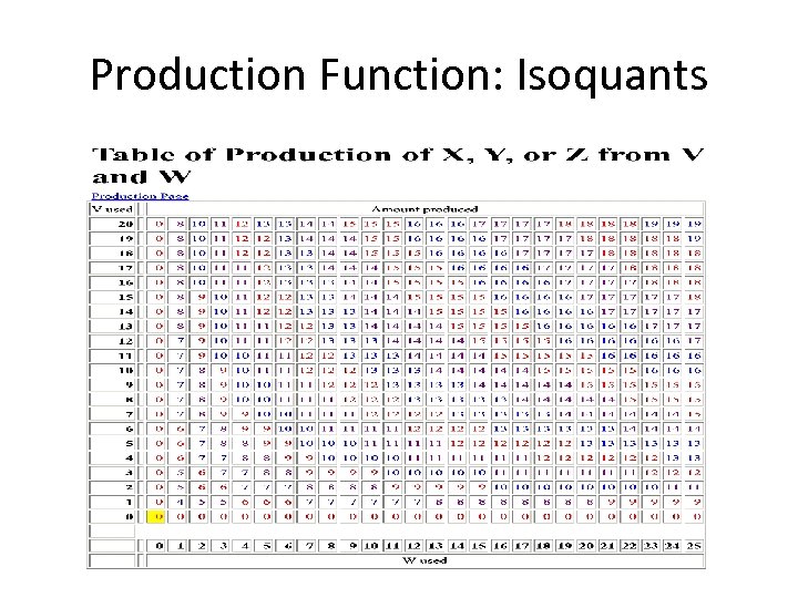
Production Function: Isoquants

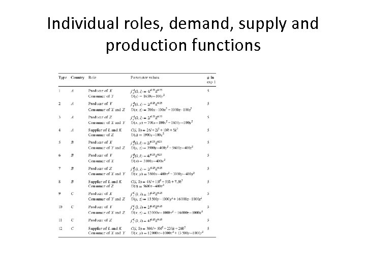
Individual roles, demand, supply and production functions

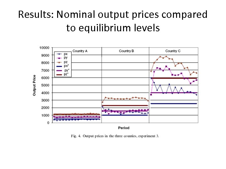
Results: Nominal output prices compared to equilibrium levels

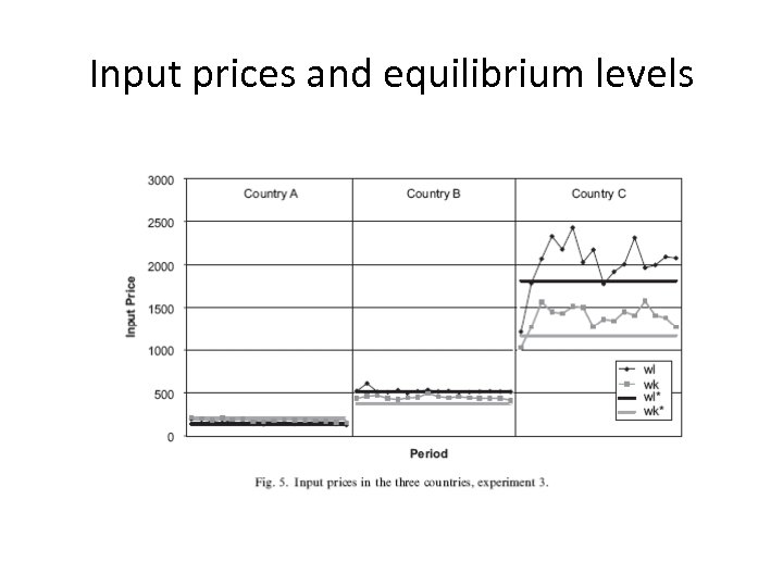
Input prices and equilibrium levels

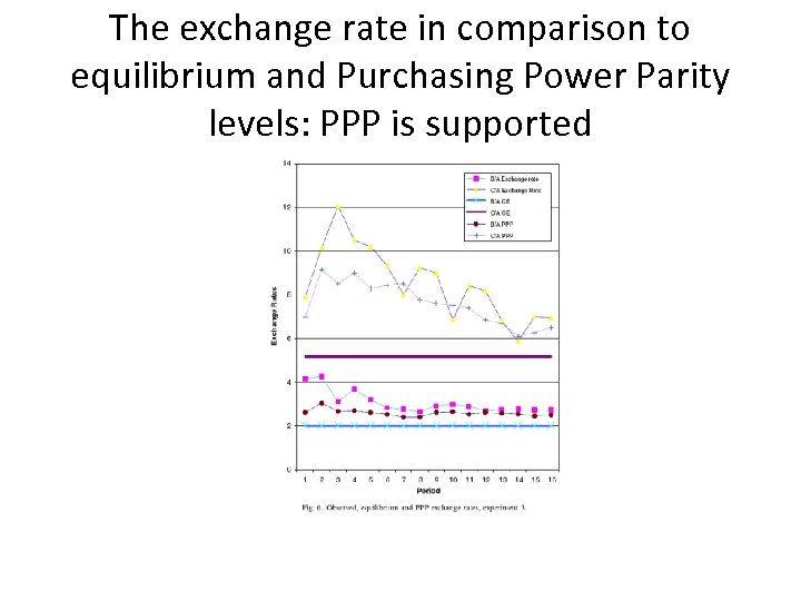
The exchange rate in comparison to equilibrium and Purchasing Power Parity levels: PPP is supported

Overall conclusions from complex economies • Equilibration, convergence to competitive equilibrium with decreasing variance, is observed. • The equilibration process appears to be slower, the more complex the economy. • It is feasible to construct and implement very complicated economies in the laboratory. • I’ll stop here: Any questions?