macro The Data of Macroeconomics Important issues

macro The Data of Macroeconomics

Important issues in macroeconomics Macroeconomics, the study of the economy as a whole, addresses many topical issues: § Why does the cost of living keep rising? § Why are millions of people unemployed, even when the economy is booming? § What causes recessions? Can the government do anything to combat recessions? Should it?

Important issues in macroeconomics Macroeconomics, the study of the economy as a whole, addresses many topical issues: § What is the government budget deficit? How does it affect the economy? § Why does the U. S. have such a huge trade deficit? § Why are so many countries poor? What policies might help them grow out of poverty?

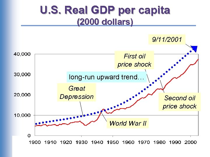U. S. Real GDP per capita (2000 dollars) 9/11/2001 First oil price shock long-run upward trend… Great Depression Second oil price shock World War II

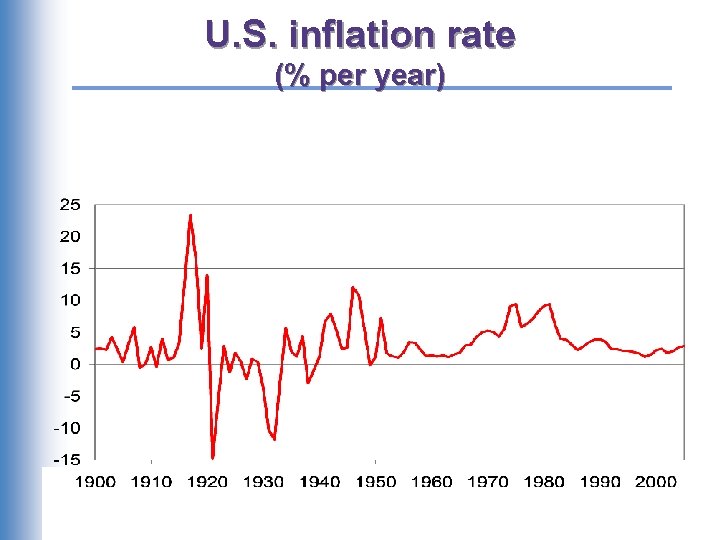U. S. inflation rate (% per year)

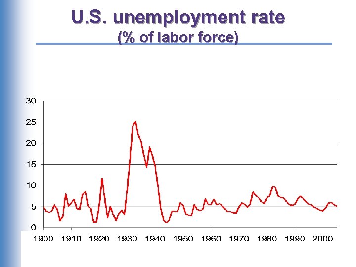U. S. unemployment rate (% of labor force)

Why learn macroeconomics? 1. The macroeconomy affects society’s wellbeing. Each one-point increase in the unemployment rate is associated with: – 920 more suicides – 650 more homicides – 4000 more people admitted to state mental institutions – 3300 more people sent to state prisons – 37, 000 more deaths – increases in domestic violence and homelessness

Why learn macroeconomics? percent change from 12 mos earlier 2. The macroeconomy affects your well-being.

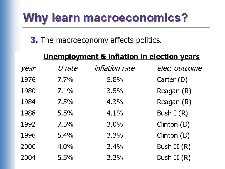Why learn macroeconomics? 3. The macroeconomy affects politics. Unemployment & inflation in election years year U rate inflation rate elec. outcome 1976 7. 7% 5. 8% Carter (D) 1980 7. 1% 13. 5% Reagan (R) 1984 7. 5% 4. 3% Reagan (R) 1988 5. 5% 4. 1% Bush I (R) 1992 7. 5% 3. 0% Clinton (D) 1996 5. 4% 3. 3% Clinton (D) 2000 4. 0% 3. 4% Bush II (R) 2004 5. 5% 3. 3% Bush II (R)

A multitude of models § So we will learn different models for studying different issues (e. g. , unemployment, inflation, long-run growth). § For each new model, you should keep track of – its assumptions – which variables are endogenous, which are exogenous – the questions it can help us understand, and those it cannot

Prices: flexible vs. sticky § Market clearing: An assumption that prices are flexible, adjust to equate supply and demand. § In the short run, many prices are sticky – adjust sluggishly in response to changes in supply or demand. For example, – many labor contracts fix the nominal wage for a year or longer – many magazine publishers change prices only once every 3 -4 years

Prices: flexible vs. sticky § The economy’s behavior depends partly on whether prices are sticky or flexible: § If prices are sticky, then demand won’t always equal supply. This helps explain – unemployment (excess supply of labor) – why firms cannot always sell all the goods they produce § Long run: prices flexible, markets clear, economy behaves very differently

Outline of this course: § Introductory material (Chaps. 1 & 2) and the Classical Theory (Chaps. 3, 4, & 6) How the economy works in the long run, when prices are flexible § Business Cycle Theory (Chaps. 9 -12) How the economy works in the short run, when prices are sticky § Policy debates (Chaps. 13 -15) Should the government try to smooth business cycle fluctuations? Is the government’s debt a problem? § Growth Theory (Chaps. 7 & 8) The standard of living and its growth rate over the very long run

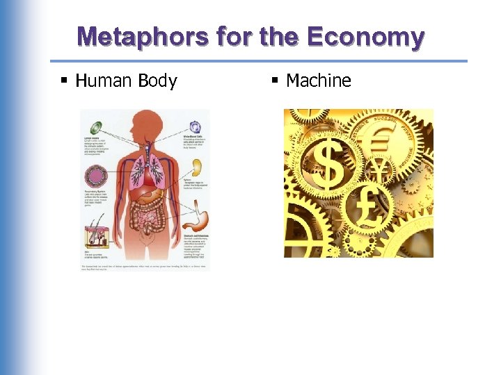Metaphors for the Economy § Human Body § Machine

macro The Data of Macroeconomics

Do you remember… …the meaning and measurement of the most important macroeconomic statistics? – Gross Domestic Product (GDP) – The Consumer Price Index (CPI) – The unemployment rate

Gross Domestic Product: Expenditure and Income Two definitions: – Total expenditure on domestically-produced final goods and services. – Total income earned by domestically-located factors of production. Expenditure equals income because every dollar spent by a buyer becomes income to the seller.

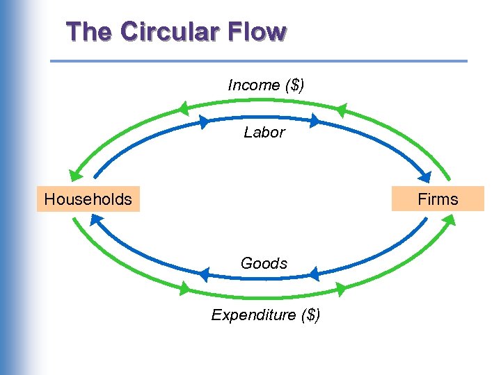The Circular Flow Income ($) Labor Firms Households Goods Expenditure ($)

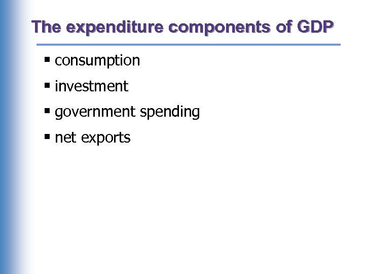The expenditure components of GDP § consumption § investment § government spending § net exports

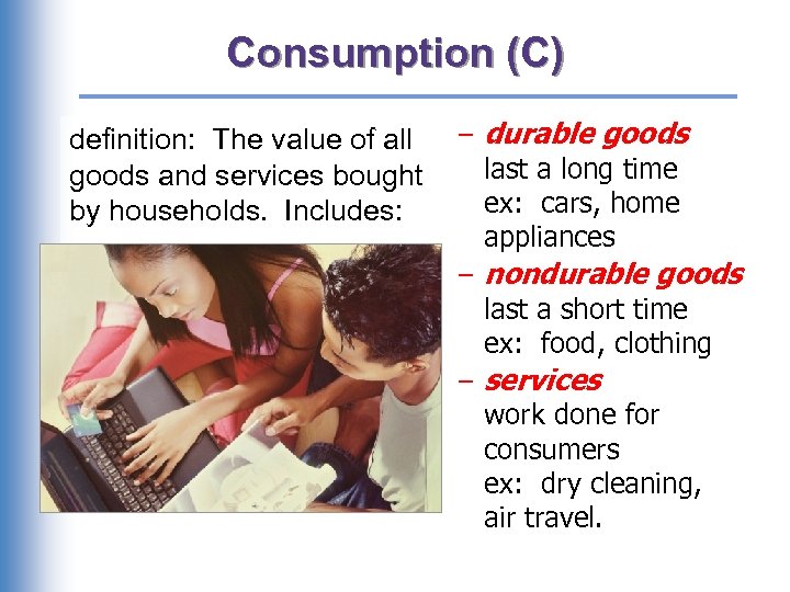Consumption (C) definition: The value of all goods and services bought by households. Includes: – durable goods last a long time ex: cars, home appliances – nondurable goods last a short time ex: food, clothing – services work done for consumers ex: dry cleaning, air travel.

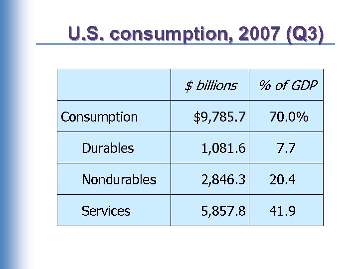U. S. consumption, 2007 (Q 3) $ billions Consumption % of GDP $9, 785. 7 70. 0% Durables 1, 081. 6 7. 7 Nondurables 2, 846. 3 20. 4 Services 5, 857. 8 41. 9

Investment (I) Definition 1: Spending on [the factor of production] capital. Definition 2: Spending on goods bought for future use Includes: – business fixed investment Spending on plant and equipment that firms will use to produce other goods & services. – residential fixed investment Spending on housing units by consumers and landlords. – inventory investment The change in the value of all firms’ inventories.

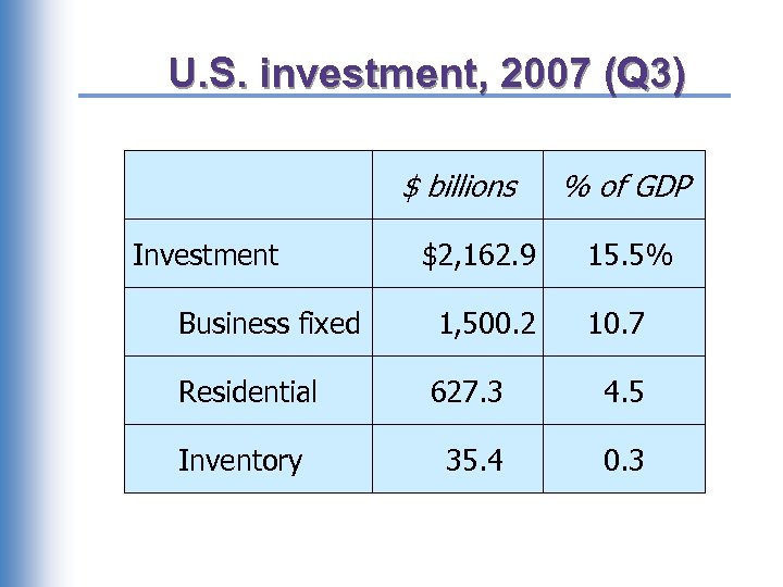U. S. investment, 2007 (Q 3) $ billions Investment $2, 162. 9 % of GDP 15. 5% Business fixed 1, 500. 2 10. 7 Residential 627. 3 4. 5 Inventory 35. 4 0. 3

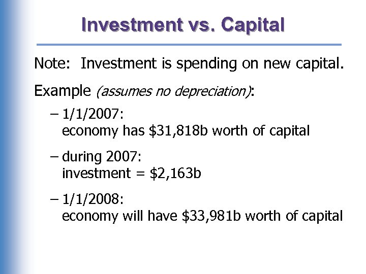Investment vs. Capital Note: Investment is spending on new capital. Example (assumes no depreciation): – 1/1/2007: economy has $31, 818 b worth of capital – during 2007: investment = $2, 163 b – 1/1/2008: economy will have $33, 981 b worth of capital

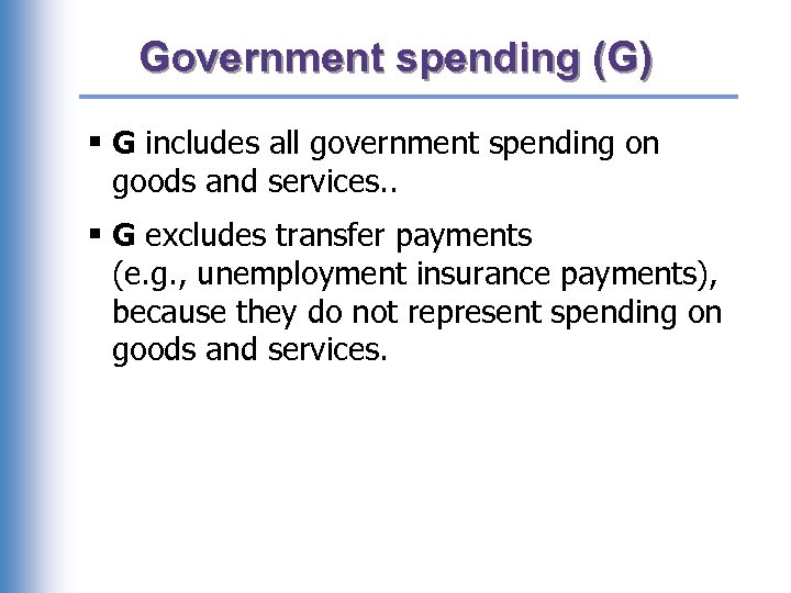Government spending (G) § G includes all government spending on goods and services. . § G excludes transfer payments (e. g. , unemployment insurance payments), because they do not represent spending on goods and services.

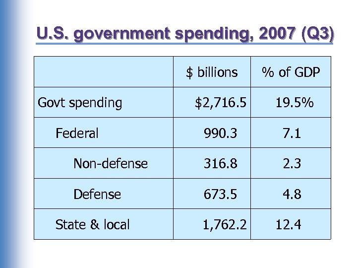U. S. government spending, 2007 (Q 3) $ billions % of GDP Govt spending $2, 716. 5 19. 5% Federal 990. 3 7. 1 Non-defense 316. 8 2. 3 Defense 673. 5 4. 8 State & local 1, 762. 2 12. 4

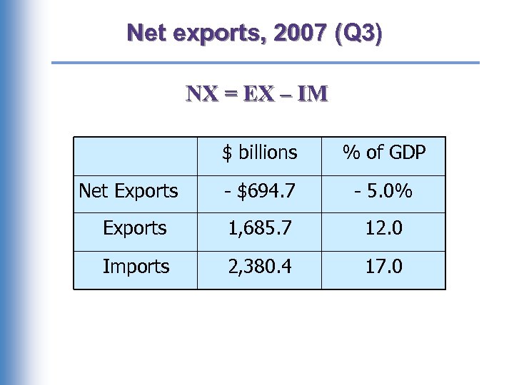Net exports, 2007 (Q 3) NX = EX – IM $ billions % of GDP - $694. 7 - 5. 0% Exports 1, 685. 7 12. 0 Imports 2, 380. 4 17. 0 Net Exports

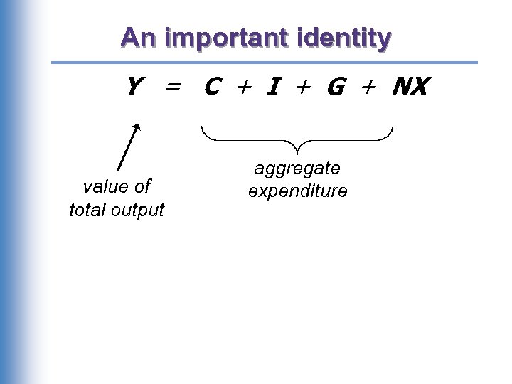An important identity Y = C + I + G + NX value of total output aggregate expenditure

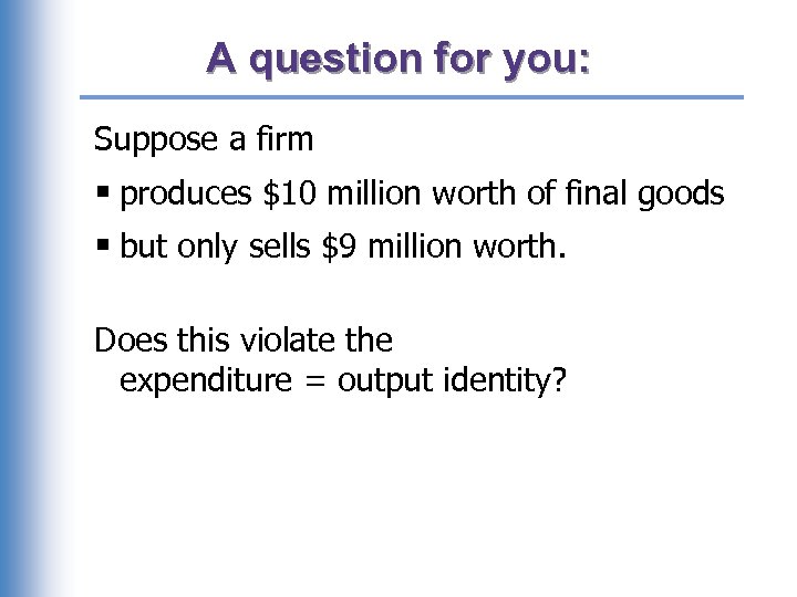A question for you: Suppose a firm § produces $10 million worth of final goods § but only sells $9 million worth. Does this violate the expenditure = output identity?

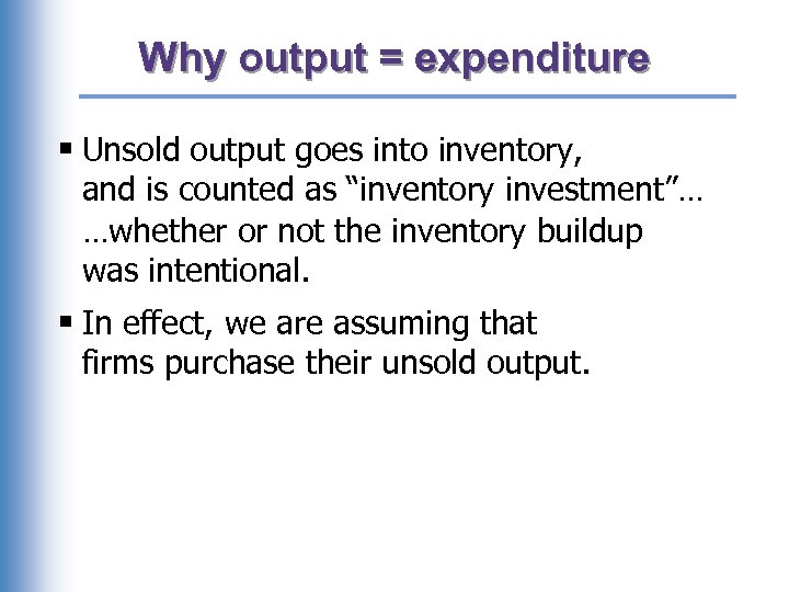Why output = expenditure § Unsold output goes into inventory, and is counted as “inventory investment”… …whether or not the inventory buildup was intentional. § In effect, we are assuming that firms purchase their unsold output.

GDP: An important and versatile concept We have now seen that GDP measures – total income – total output – total expenditure

GNP vs. GDP § Gross National Product (GNP): Total income earned by the nation’s factors of production, regardless of where located. § Gross Domestic Product (GDP): Total income earned by domestically-located factors of production, regardless of nationality.

Discussion question: In your country, which would you want to be bigger, GDP, or GNP? Why?

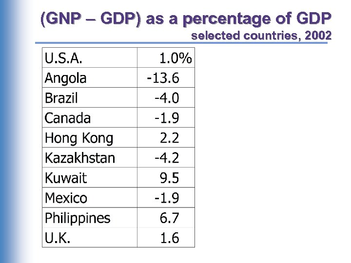(GNP – GDP) as a percentage of GDP selected countries, 2002

Real vs. nominal GDP § GDP is the value of all final goods and services produced. § nominal GDP measures these values using current prices. § real GDP measure these values using the prices of a base year.

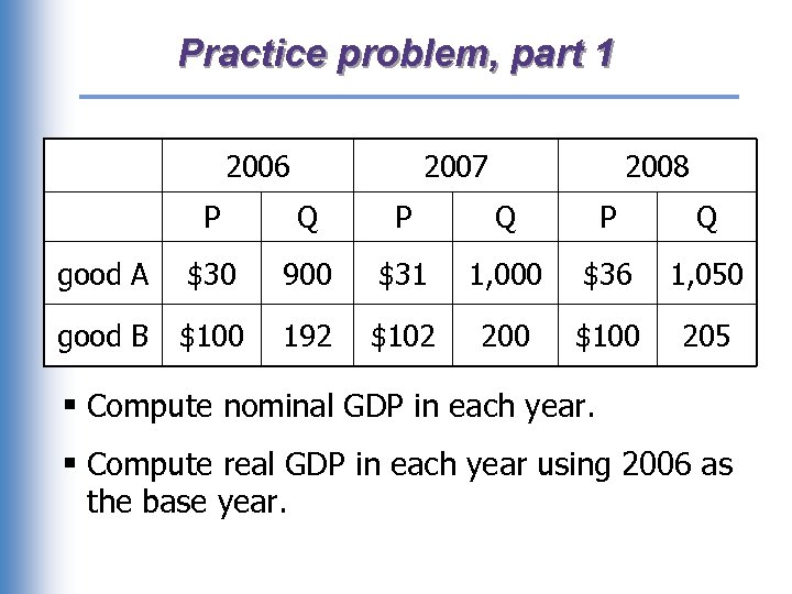Practice problem, part 1 2006 2007 2008 P Q P Q good A $30 900 $31 1, 000 $36 1, 050 good B $100 192 $102 200 $100 205 § Compute nominal GDP in each year. § Compute real GDP in each year using 2006 as the base year.

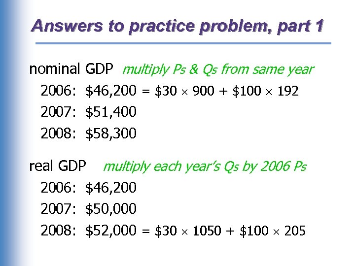Answers to practice problem, part 1 nominal 2006: 2007: 2008: GDP multiply Ps & Qs from same year $46, 200 = $30 900 + $100 192 $51, 400 $58, 300 real GDP multiply each year’s Qs by 2006 Ps 2006: $46, 2007: $50, 000 2008: $52, 000 = $30 1050 + $100 205

Real GDP controls for inflation Changes in nominal GDP can be due to: – changes in prices. – changes in quantities of output produced. Changes in real GDP can only be due to changes in quantities, because real GDP is constructed using constant base-year prices.

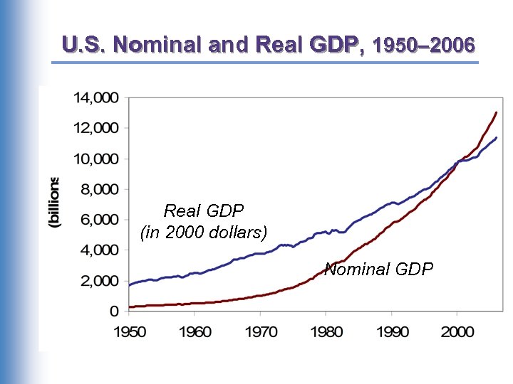U. S. Nominal and Real GDP, 1950– 2006 Real GDP (in 2000 dollars) Nominal GDP

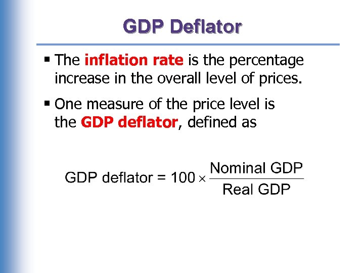GDP Deflator § The inflation rate is the percentage increase in the overall level of prices. § One measure of the price level is the GDP deflator, defined as

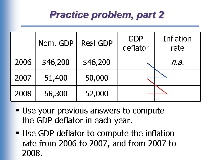Practice problem, part 2 Nom. GDP Real GDP 2006 $46, 200 51, 400 58, 300 n. a. 50, 000 2008 Inflation rate $46, 2007 GDP deflator 52, 000 § Use your previous answers to compute the GDP deflator in each year. § Use GDP deflator to compute the inflation rate from 2006 to 2007, and from 2007 to 2008.

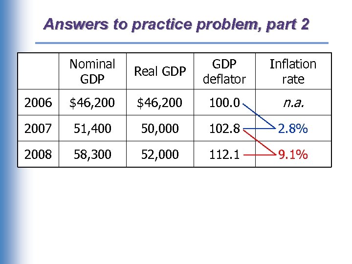Answers to practice problem, part 2 Nominal GDP Real GDP deflator Inflation rate 2006 $46, 200 100. 0 n. a. 2007 51, 400 50, 000 102. 8% 2008 58, 300 52, 000 112. 1 9. 1%

Consumer Price Index (CPI) § A measure of the overall level of prices § Published by the Bureau of Labor Statistics (BLS) § Uses: – tracks changes in the typical household’s cost of living – adjusts many contracts for inflation (“COLAs”) – allows comparisons of dollar amounts over time

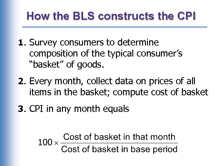How the BLS constructs the CPI 1. Survey consumers to determine composition of the typical consumer’s “basket” of goods. 2. Every month, collect data on prices of all items in the basket; compute cost of basket 3. CPI in any month equals

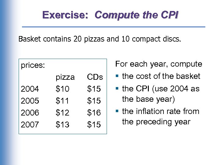Exercise: Compute the CPI Basket contains 20 pizzas and 10 compact discs. For each year, compute prices: 2004 2005 2006 2007 pizza $10 $11 $12 $13 CDs $15 $16 $15 § the cost of the basket § the CPI (use 2004 as the base year) § the inflation rate from the preceding year

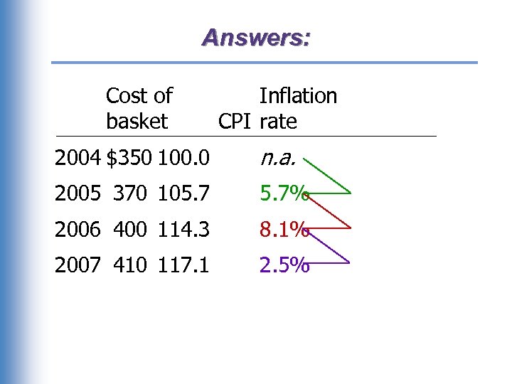Answers: Cost of basket Inflation CPI rate 2004 $350 100. 0 n. a. 2005 370 105. 7% 2006 400 114. 3 8. 1% 2007 410 117. 1 2. 5%

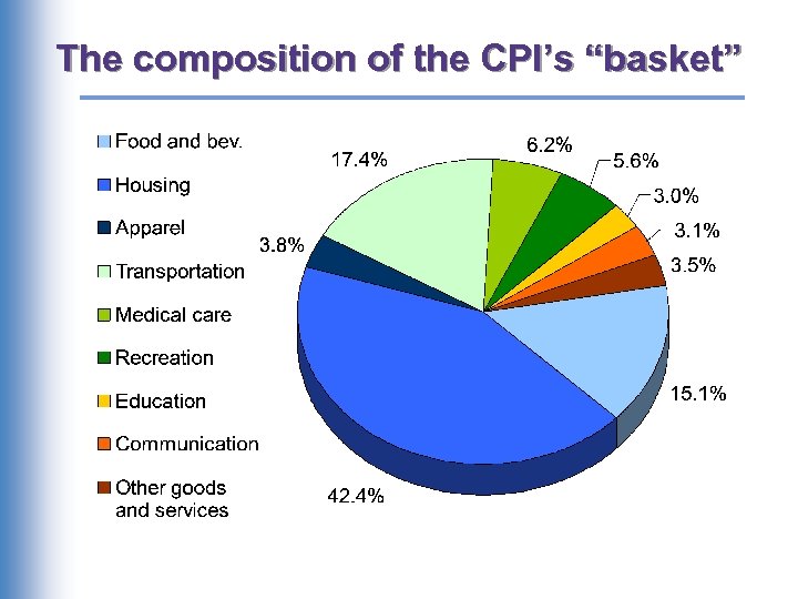The composition of the CPI’s “basket”

Reasons why the CPI may overstate inflation § Substitution bias: The CPI uses fixed weights, so it cannot reflect consumers’ ability to substitute toward goods whose relative prices have fallen. § Introduction of new goods: The introduction of new goods makes consumers better off and, in effect, increases the real value of the dollar. But it does not reduce the CPI, because the CPI uses fixed weights. § Unmeasured changes in quality: Quality improvements increase the value of the dollar, but are often not fully measured.

The size of the CPI’s bias § In 1995, a Senate-appointed panel of experts estimated that the CPI overstates inflation by about 1. 1% per year. § Now, the CPI’s bias is probably under 1% per year.

CPI vs. GDP Deflator prices of capital goods – included in GDP deflator (if produced domestically) – excluded from CPI prices of imported consumer goods – included in CPI – excluded from GDP deflator the basket of goods – CPI: fixed – GDP deflator: changes every year

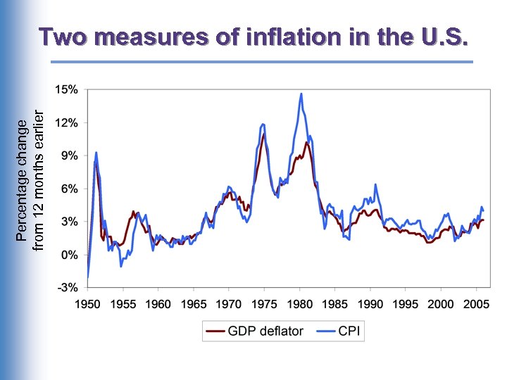Percentage change from 12 months earlier Two measures of inflation in the U. S.

Labor Market Data § Household survey (60, 000 HH) § Employer survey (160, 000 B+GA)

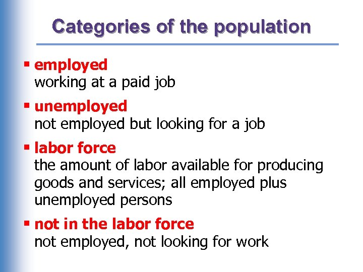Categories of the population § employed working at a paid job § unemployed not employed but looking for a job § labor force the amount of labor available for producing goods and services; all employed plus unemployed persons § not in the labor force not employed, not looking for work

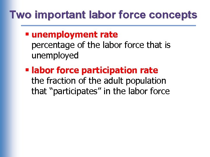Two important labor force concepts § unemployment rate percentage of the labor force that is unemployed § labor force participation rate the fraction of the adult population that “participates” in the labor force

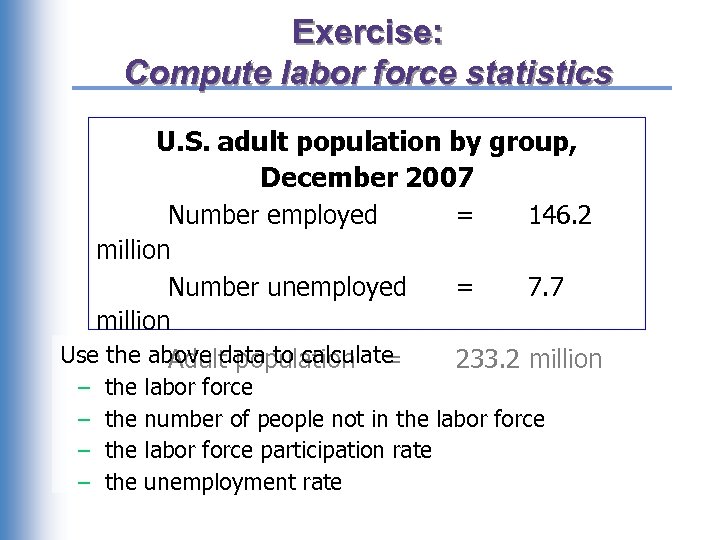Exercise: Compute labor force statistics U. S. adult population by group, December 2007 Number employed = 146. 2 million Number unemployed = 7. 7 million Use the above data to calculate Adult population = 233. 2 million – – the the labor force number of people not in the labor force participation rate unemployment rate

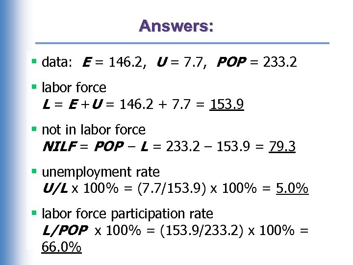Answers: § data: E = 146. 2, U = 7. 7, POP = 233. 2 § labor force L = E +U = 146. 2 + 7. 7 = 153. 9 § not in labor force NILF = POP – L = 233. 2 – 153. 9 = 79. 3 § unemployment rate U/L x 100% = (7. 7/153. 9) x 100% = 5. 0% § labor force participation rate L/POP x 100% = (153. 9/233. 2) x 100% = 66. 0%

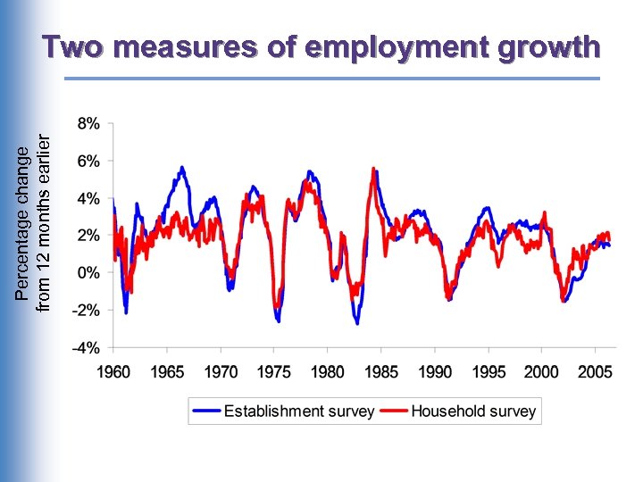Percentage change from 12 months earlier Two measures of employment growth

macro A Long Run Model: Where Income Comes From and Where it Goes

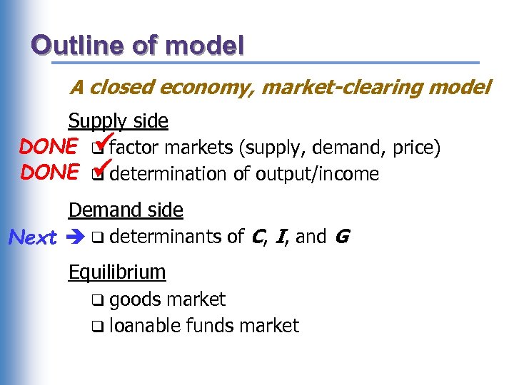
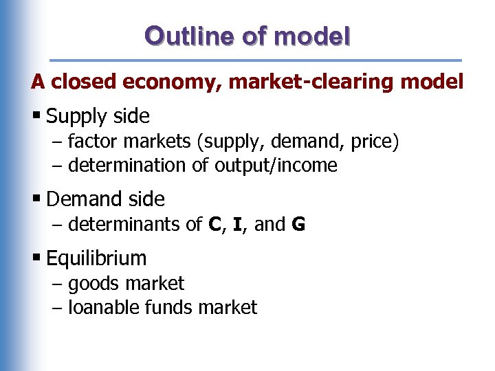Outline of model A closed economy, market-clearing model § Supply side – factor markets (supply, demand, price) – determination of output/income § Demand side – determinants of C, I, and G § Equilibrium – goods market – loanable funds market

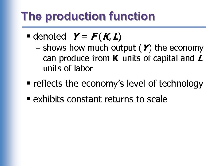The production function § denoted Y = F (K, L) – shows how much output (Y ) the economy can produce from K units of capital and L units of labor § reflects the economy’s level of technology § exhibits constant returns to scale

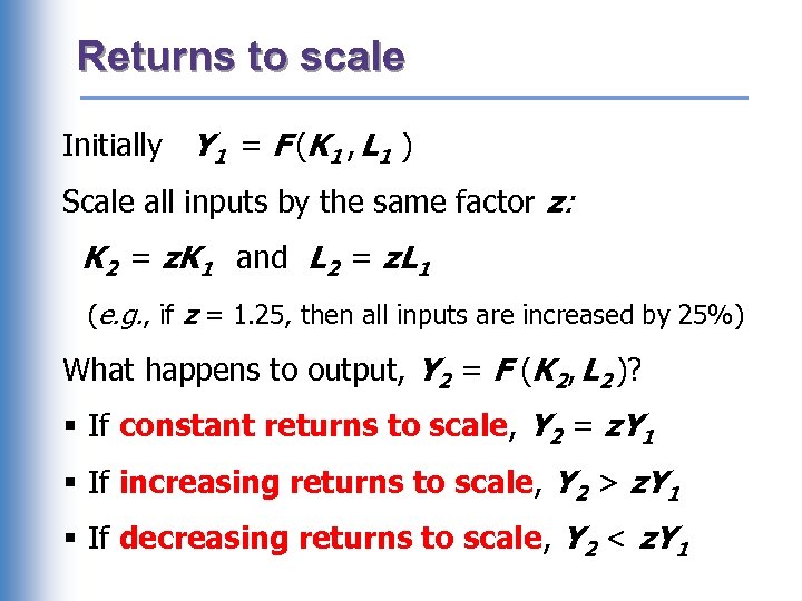Returns to scale Initially Y 1 = F (K 1 , L 1 ) Scale all inputs by the same factor z: K 2 = z. K 1 and L 2 = z. L 1 (e. g. , if z = 1. 25, then all inputs are increased by 25%) What happens to output, Y 2 = F (K 2, L 2 )? § If constant returns to scale, Y 2 = z. Y 1 § If increasing returns to scale, Y 2 > z. Y 1 § If decreasing returns to scale, Y 2 < z. Y 1

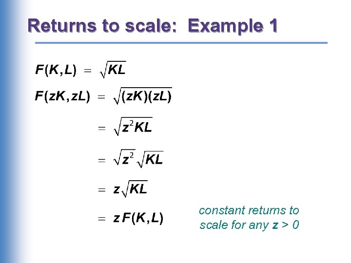Returns to scale: Example 1 constant returns to scale for any z > 0

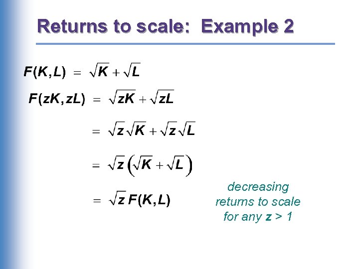Returns to scale: Example 2 decreasing returns to scale for any z > 1

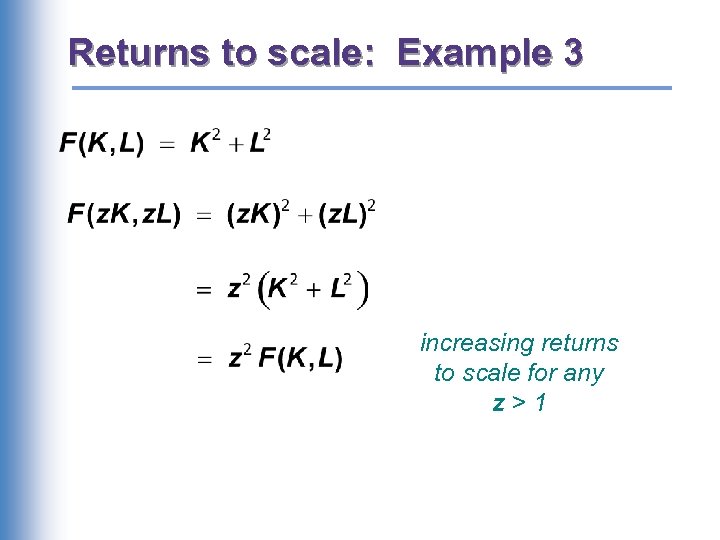Returns to scale: Example 3 increasing returns to scale for any z>1

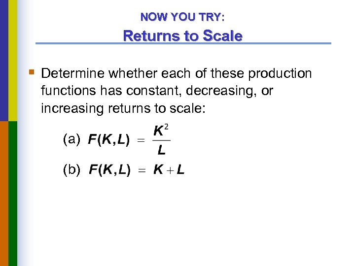NOW YOU TRY: Returns to Scale § Determine whether each of these production functions has constant, decreasing, or increasing returns to scale: (a) (b)

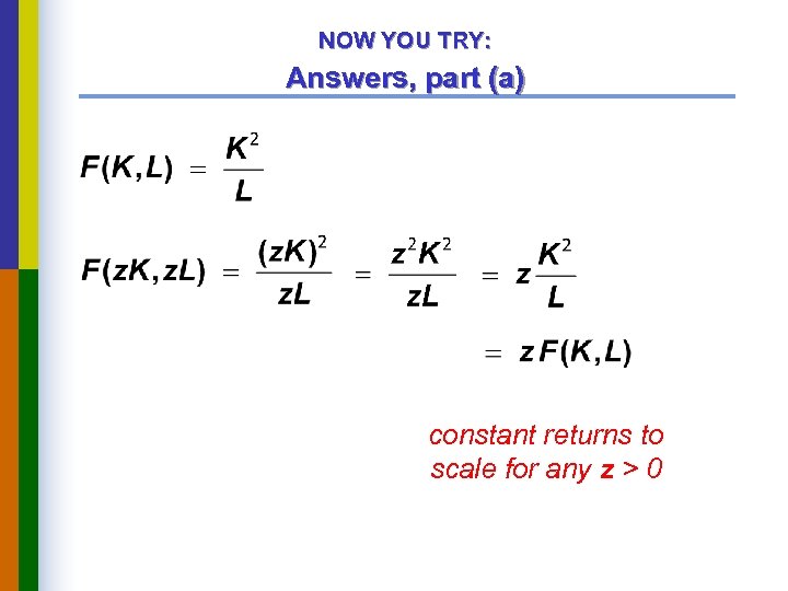NOW YOU TRY: Answers, part (a) constant returns to scale for any z > 0

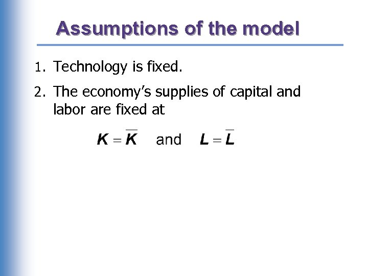Assumptions of the model 1. Technology is fixed. 2. The economy’s supplies of capital and labor are fixed at

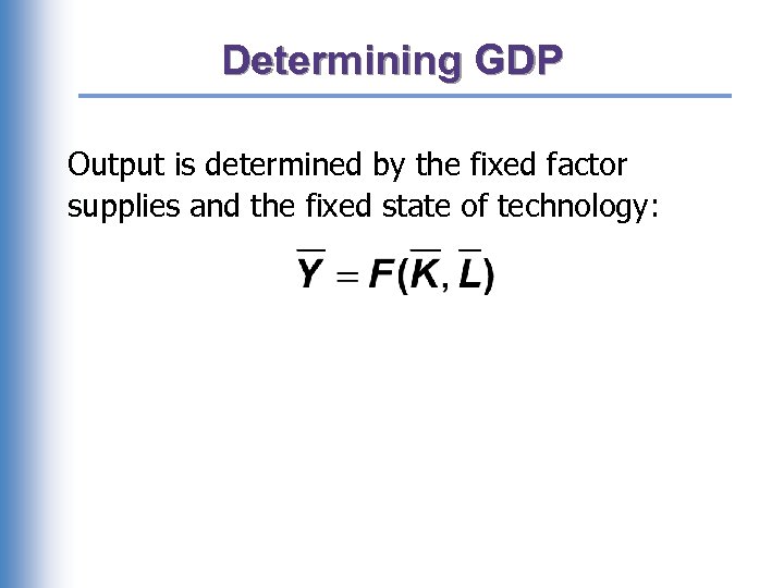Determining GDP Output is determined by the fixed factor supplies and the fixed state of technology:

The distribution of national income § determined by factor prices, the prices per unit firms pay for the factors of production – wage = price of L – rental rate = price of K

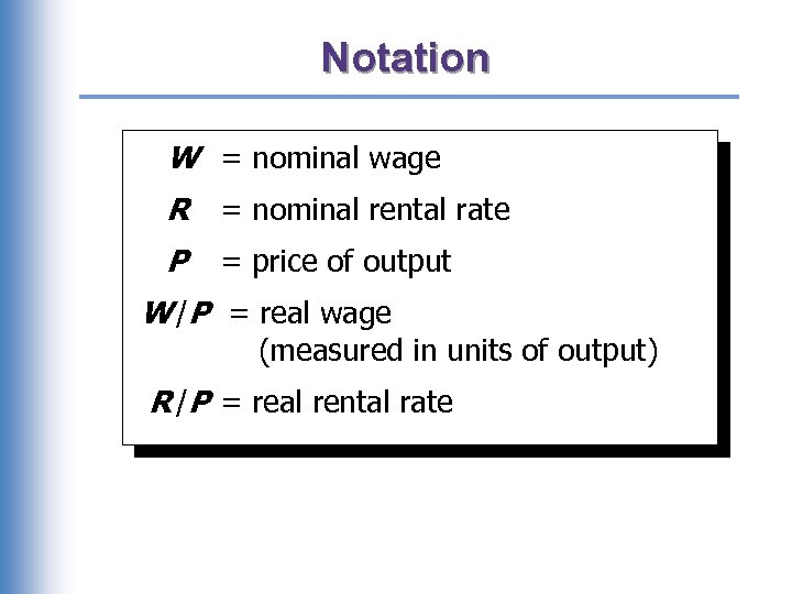Notation W = nominal wage R = nominal rental rate P = price of output W /P = real wage (measured in units of output) R /P = real rental rate

How factor prices are determined § Factor prices are determined by supply and demand in factor markets. § Recall: Supply of each factor is fixed. § What about demand?

Demand for labor § Assume markets are competitive: each firm takes W, R, and P as given. § Basic idea: A firm hires each unit of labor if the cost does not exceed the benefit. – cost = real wage – benefit = marginal product of labor

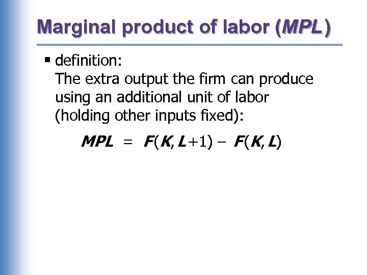Marginal product of labor (MPL ) § definition: The extra output the firm can produce using an additional unit of labor (holding other inputs fixed): MPL = F (K, L +1) – F (K, L)

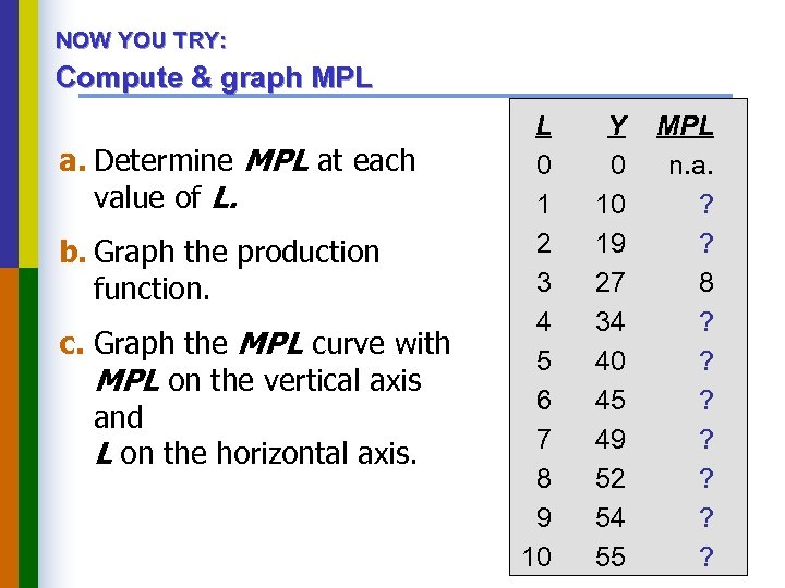NOW YOU TRY: Compute & graph MPL a. Determine MPL at each value of L. b. Graph the production function. c. Graph the MPL curve with MPL on the vertical axis and L on the horizontal axis. L 0 1 2 3 4 5 6 7 8 9 10 Y 0 10 19 27 34 40 45 49 52 54 55 MPL n. a. ? ? 8 ? ? ? ?

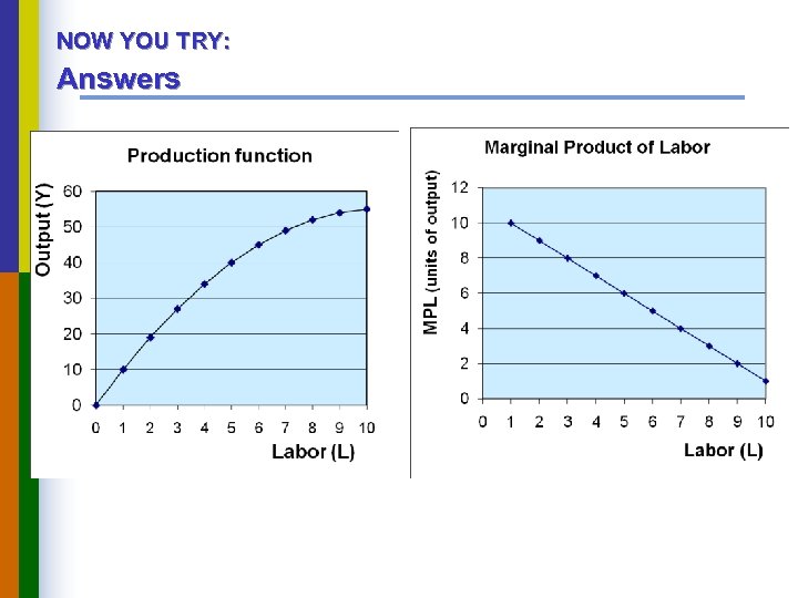NOW YOU TRY: Answers

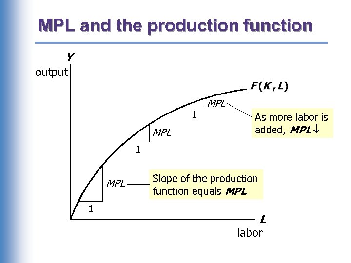MPL and the production function Y output 1 MPL As more labor is added, MPL 1 MPL 1 Slope of the production function equals MPL L labor

Diminishing marginal returns § As a factor input is increased, its marginal product falls (ceteris paribus). § Intuition: Suppose L while holding K fixed fewer machines per worker lower worker productivity

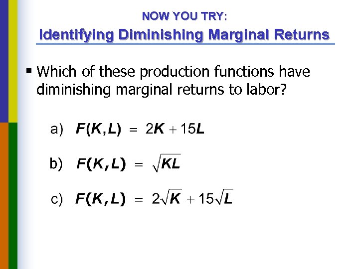NOW YOU TRY: Identifying Diminishing Marginal Returns § Which of these production functions have diminishing marginal returns to labor?

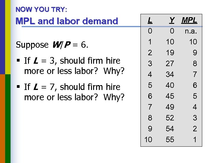NOW YOU TRY: MPL and labor demand Suppose W/P = 6. § If L = 3, should firm hire more or less labor? Why? § If L = 7, should firm hire more or less labor? Why? L 0 1 2 3 4 5 6 7 8 9 10 Y MPL 0 n. a. 10 10 19 9 27 8 34 7 40 6 45 5 49 4 52 3 54 2 55 1

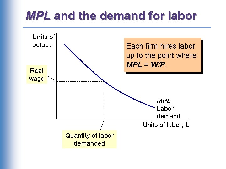MPL and the demand for labor Units of output Each firm hires labor up to the point where MPL = W/P. Real wage MPL, Labor demand Units of labor, L Quantity of labor demanded

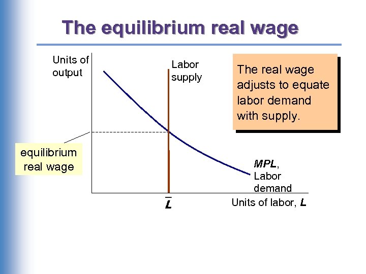The equilibrium real wage Units of output equilibrium real wage Labor supply The real wage adjusts to equate labor demand with supply. MPL, Labor demand Units of labor, L

Determining the rental rate § We have just seen that MPL = W/P. § The same logic shows that MPK = R/P : – diminishing returns to capital: MPK as K – The MPK curve is the firm’s demand curve for renting capital. – Firms maximize profits by choosing K such that MPK = R/P.

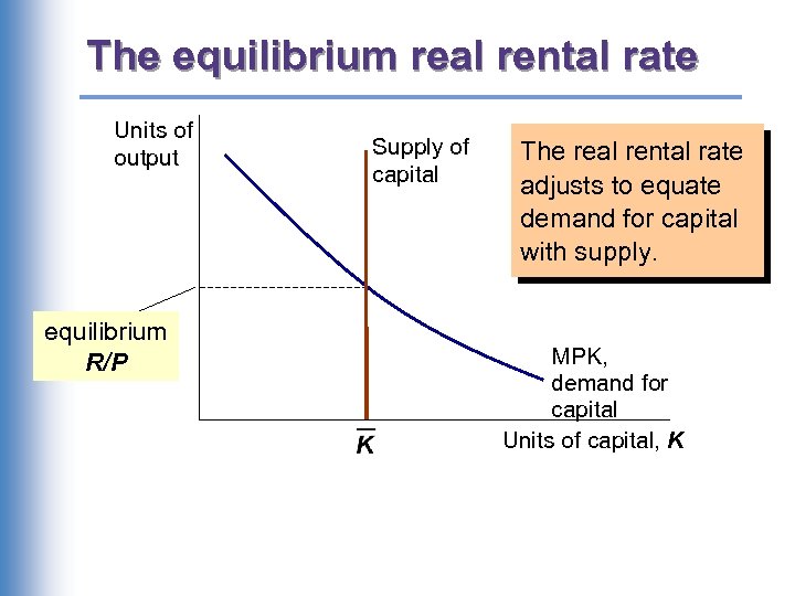The equilibrium real rental rate Units of output equilibrium R/P Supply of capital The real rental rate adjusts to equate demand for capital with supply. MPK, demand for capital Units of capital, K

The Neoclassical Theory of Distribution § states that each factor input is paid its marginal product § a good starting point for thinking about income distribution

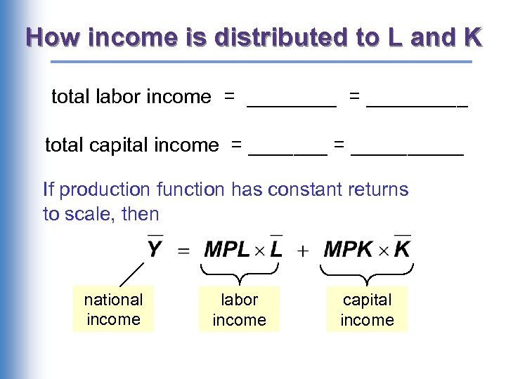How income is distributed to L and K total labor income = _________ total capital income = __________ If production function has constant returns to scale, then national income labor income capital income

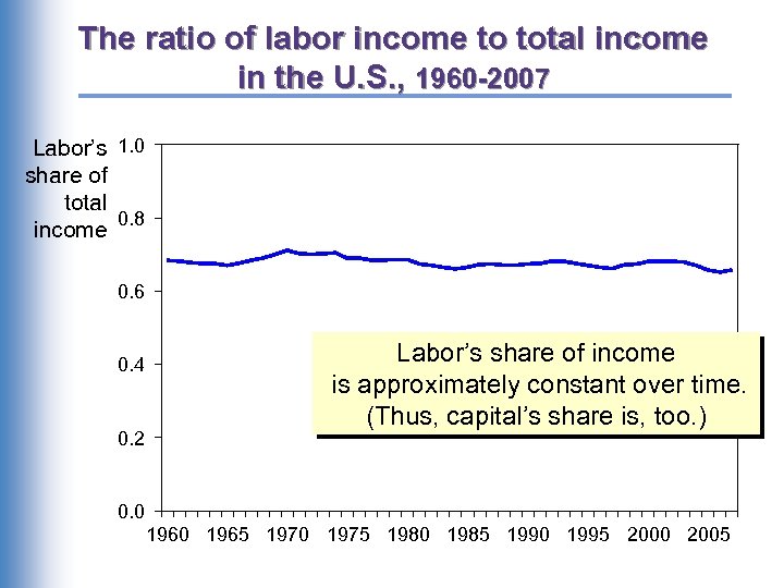The ratio of labor income to total income in the U. S. , 1960 -2007 Labor’s 1. 0 share of total 0. 8 income 0. 6 0. 4 0. 2 Labor’s share of income is approximately constant over time. (Thus, capital’s share is, too. ) 0. 0 1965 1970 1975 1980 1985 1990 1995 2000 2005

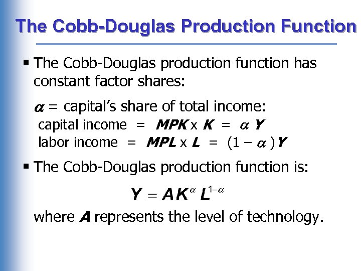The Cobb-Douglas Production Function § The Cobb-Douglas production function has constant factor shares: = capital’s share of total income: capital income = MPK x K = Y labor income = MPL x L = (1 – )Y § The Cobb-Douglas production function is: where A represents the level of technology.

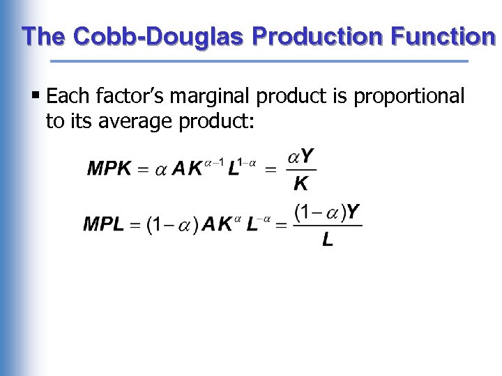The Cobb-Douglas Production Function § Each factor’s marginal product is proportional to its average product:

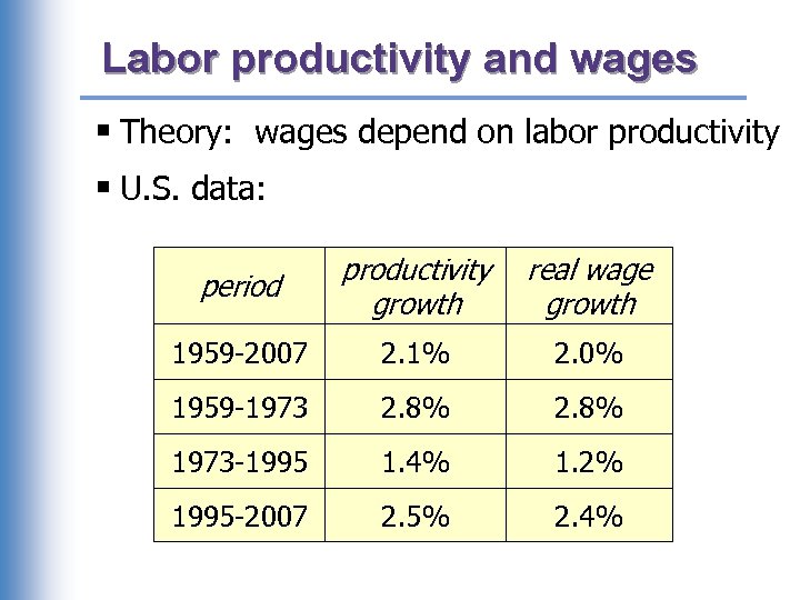Labor productivity and wages § Theory: wages depend on labor productivity § U. S. data: period productivity growth real wage growth 1959 -2007 2. 1% 2. 0% 1959 -1973 2. 8% 1973 -1995 1. 4% 1. 2% 1995 -2007 2. 5% 2. 4%

Outline of model A closed economy, market-clearing model Supply side DONE q factor markets (supply, demand, price) DONE q determination of output/income Demand side Next q determinants of C, I, and G Equilibrium q goods market q loanable funds market

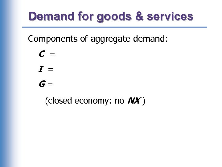Demand for goods & services Components of aggregate demand: C = I = G= (closed economy: no NX )

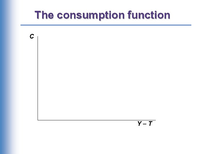
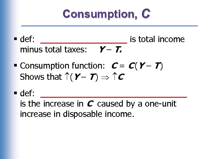Consumption, C § def: ________ is total income minus total taxes: Y – T. § Consumption function: C = C (Y – T ) Shows that (Y – T ) C § def: ______________ is the increase in C caused by a one-unit increase in disposable income.

The consumption function C Y–T

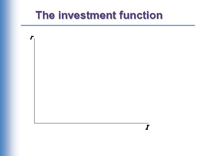
Investment, I § The investment function is I = I (r ), where r denotes the _________, the nominal interest rate corrected for inflation. § The real interest rate is – ________________________________. So, r I

The investment function r I

Government spending, G § G = govt spending on goods and services. § G excludes ____________ (e. g. , social security benefits, unemployment insurance benefits). § Assume government spending and total taxes are exogenous:

The market for goods & services § Aggregate demand: § Aggregate supply: § Equilibrium: § The __________ adjusts to equate demand with supply.

The loanable funds market § A simple supply-demand model of the financial system. § One asset: “loanable funds” – demand for funds: _________ – supply of funds: _________ – “price” of funds: _________

Demand for funds: Investment The demand for loanable funds… – _______________: Firms borrow to finance spending on plant & equipment, new office buildings, etc. Consumers borrow to buy new houses. – _______________, the “price” of loanable funds (cost of borrowing).

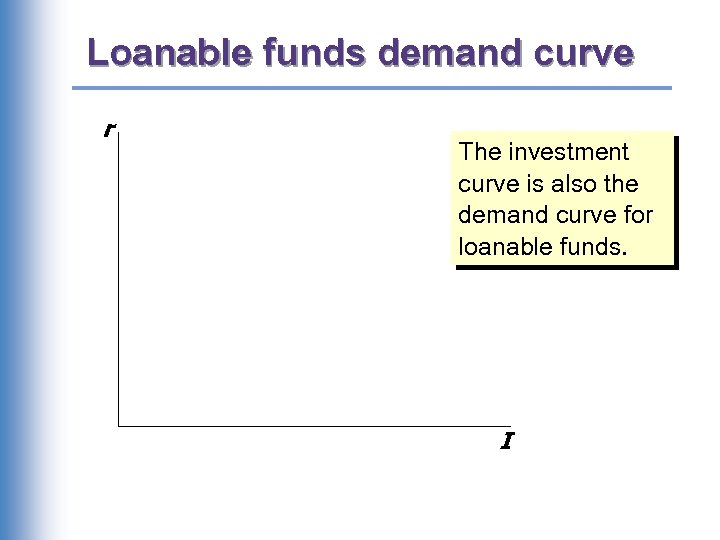Loanable funds demand curve r The investment curve is also the demand curve for loanable funds. I

Supply of funds: Saving § The supply of loanable funds comes from saving: – ________________________________

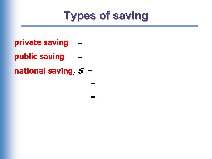Types of saving private saving = public saving = national saving, S = = =

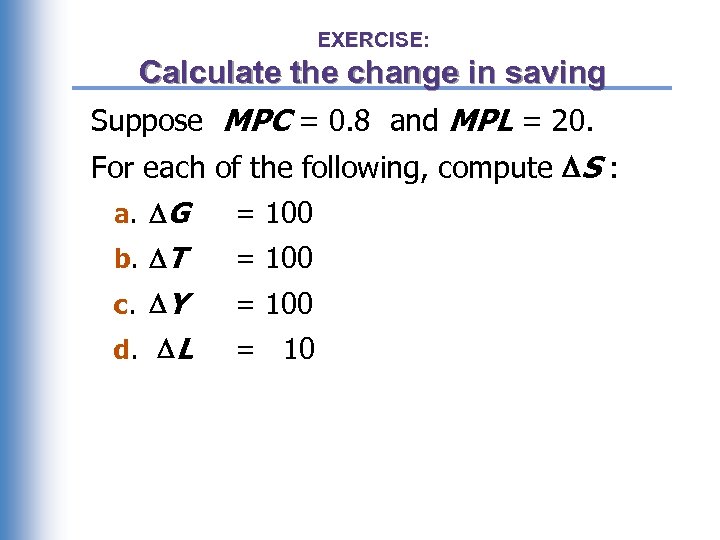EXERCISE: Calculate the change in saving Suppose MPC = 0. 8 and MPL = 20. For each of the following, compute S : a. G = 100 b. T = 100 c. Y = 100 d. L = 10

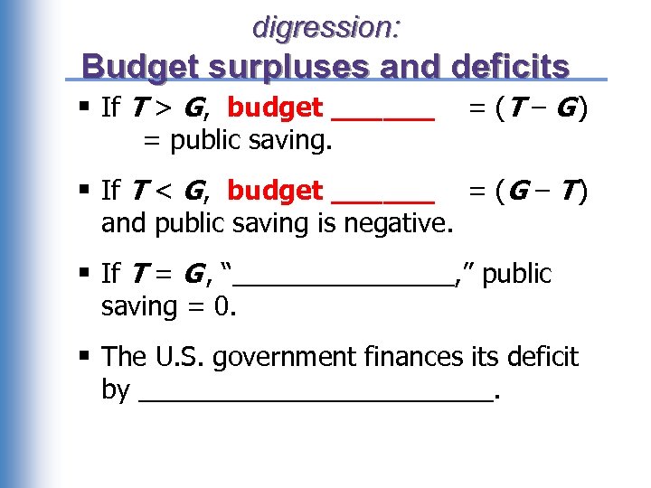digression: Budget surpluses and deficits § If T > G, budget ______ = (T – G ) § If T < G, budget ______ = (G – T ) = public saving. and public saving is negative. § If T = G , “________, ” public saving = 0. § The U. S. government finances its deficit by ____________.

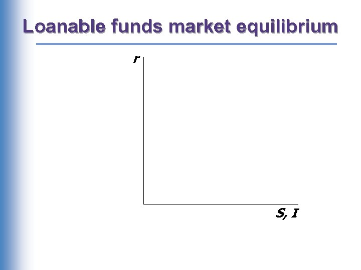Loanable funds market equilibrium r S, I

The special role of r r adjusts to equilibrate the _______ market and the ________ market simultaneously:

Mastering the loanable funds model Things that shift the saving curve: Things that shift the investment curve

CASE STUDY: The Reagan deficits § Reagan policies during early 1980 s: – ____________________________ § Both policies reduce national saving:

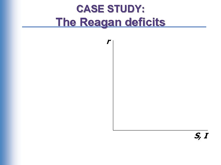CASE STUDY: The Reagan deficits r S, I

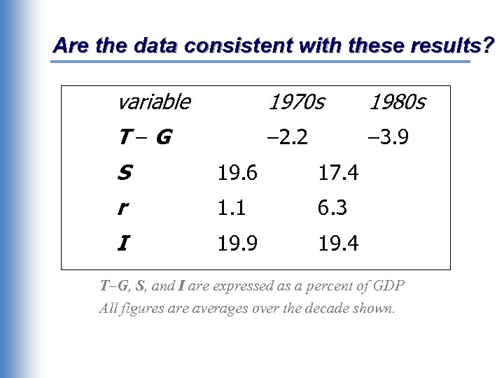Are the data consistent with these results? variable 1970 s 1980 s T–G – 2. 2 – 3. 9 S 19. 6 17. 4 r 1. 1 6. 3 I 19. 9 19. 4 T–G, S, and I are expressed as a percent of GDP All figures are averages over the decade shown.

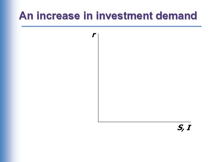An increase in investment demand r S, I

Saving and the interest rate § Why might saving depend on r ? § How would the results of an increase in investment demand be different? – Would r rise as much? – Would the equilibrium value of I change?