MACRO REVIEW in preparation for API 120 I

MACRO REVIEW in preparation for API 120 (I) DEFINITIONS & ACCOUNTING (i) National income & product accounts (ii) Balance of Payments accounts (II) THE KEYNESIAN MODEL API-120 - Macroeconomic Policy Analysis I , Prof. J. Frankel, Harvard Kennedy School

(i) National income & product accounts • Definition of macroeconomics – Aggregates – Goods (& labor) markets don’t clear in short run – Role for monetary & fiscal policy. • Definition of – GDP – GNP (includes profits of MNCs abroad) – National Income (includes unilateral transfers) API-120 - Macroeconomic Policy Analysis I , Prof. J. Frankel, Harvard Kennedy School

Ways to decompose GDP • To whom the goods & services (GDP) are sold: – – C I G X-M • How the income (Y) is used: – Taxes net of transfers, gives disposable income – Saving – Consumption • Allocation of shares according to factors of production – Wages & salaries – Capital income – Self-employed and other API-120 - Macroeconomic Policy Analysis I , Prof. J. Frankel, Harvard Kennedy School

(ii) Balance of Payments accounts • Definition: The balance of payments is the year’s record of economic transactions between domestic & foreign residents. • The rules: – If you have to pay a foreign resident, normally in exchange for something that you bring into the country, then the something counts as a debit. – If a foreign resident has to pay you for something, then the something counts as a credit. API-120 , Prof. J. Frankel, Harvard Kennedy School

† † Now also called “financial account” API-120 , Prof. J. Frankel, Harvard Kennedy School

The rules, continued • Each transactions is recorded twice: once as a credit and once as a debit. – E. g. , when an importer pays cash dollars, • the debit on the merchandise account is offset by • a credit under short-term capital: the exporter in the other country has, at least for the moment, increased holdings of US assets, which counts as a credit just like any other portfolio investment in US assets. • At the end of each quarter, credits and debits are added up within each line-item; • and line-items are cumulated from the top to compute measures of external balance.

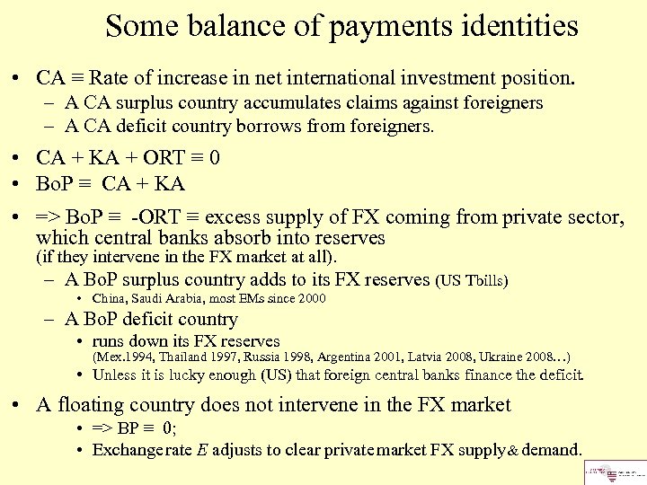Some balance of payments identities • CA ≡ Rate of increase in net international investment position. – A CA surplus country accumulates claims against foreigners – A CA deficit country borrows from foreigners. • CA + KA + ORT ≡ 0 • Bo. P ≡ CA + KA • => Bo. P ≡ -ORT ≡ excess supply of FX coming from private sector, which central banks absorb into reserves (if they intervene in the FX market at all). – A Bo. P surplus country adds to its FX reserves (US Tbills) • China, Saudi Arabia, most EMs since 2000 – A Bo. P deficit country • runs down its FX reserves (Mex. 1994, Thailand 1997, Russia 1998, Argentina 2001, Latvia 2008, Ukraine 2008…) • Unless it is lucky enough (US) that foreign central banks finance the deficit. • A floating country does not intervene in the FX market • => BP ≡ 0; • Exchange rate E adjusts to clear private market FX supply & demand.

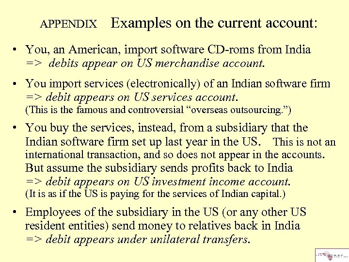APPENDIX Examples on the current account: • You, an American, import software CD-roms from India => debits appear on US merchandise account. • You import services (electronically) of an Indian software firm => debit appears on US services account. (This is the famous and controversial “overseas outsourcing. ”) • You buy the services, instead, from a subsidiary that the Indian software firm set up last year in the US. This is not an international transaction, and so does not appear in the accounts. But assume the subsidiary sends profits back to India => debit appears on US investment income account. (It is as if the US is paying for the services of Indian capital. ) • Employees of the subsidiary in the US (or any other US resident entities) send money to relatives back in India => debit appears under unilateral transfers.

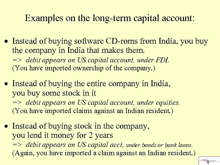Examples on the long-term capital account: Instead of buying software CD-roms from India, you buy the company in India that makes them. => debit appears on US capital account, under FDI. (You have imported ownership of the company. ) Instead of buying the entire company in India, you buy some stock in it => debit appears on US capital account, under equities. (You have imported claims against an Indian resident. ) Instead of buying stock in the company, you lend it money for 2 years => debit appears on US capital acct, under bonds or bank loans. (Again, you have imported a claim against an Indian resident. )

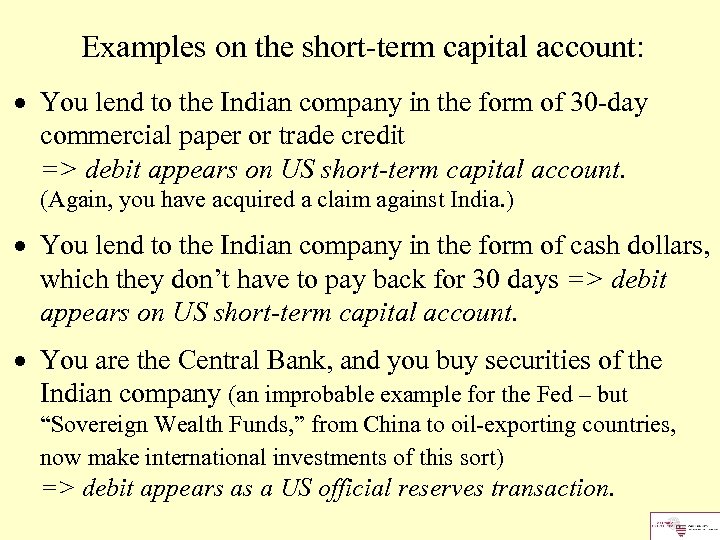Examples on the short-term capital account: You lend to the Indian company in the form of 30 -day commercial paper or trade credit => debit appears on US short-term capital account. (Again, you have acquired a claim against India. ) You lend to the Indian company in the form of cash dollars, which they don’t have to pay back for 30 days => debit appears on US short-term capital account. You are the Central Bank, and you buy securities of the Indian company (an improbable example for the Fed – but “Sovereign Wealth Funds, ” from China to oil-exporting countries, now make international investments of this sort) => debit appears as a US official reserves transaction.

End of: Definitions & Accounting API-120 - Macroeconomic Policy Analysis, Prof. Jeffrey Frankel, Harvard Kennedy School

MACRO REVIEW (II) THE KEYNESIAN MODEL Part 1: Introduction to Keynesian Model: Derivation, and National Saving Identity. Part 2: Multipliers for spending & exports Part 3: International transmission under fixed vs. floating exchange rates Part 4: Adjustment of a CA deficit via expenditure-reducing vs. expenditure-switching policies Part 5: Monetary factors API-120 - Macroeconomic Policy Analysis I , Professor Jeffrey Frankel,

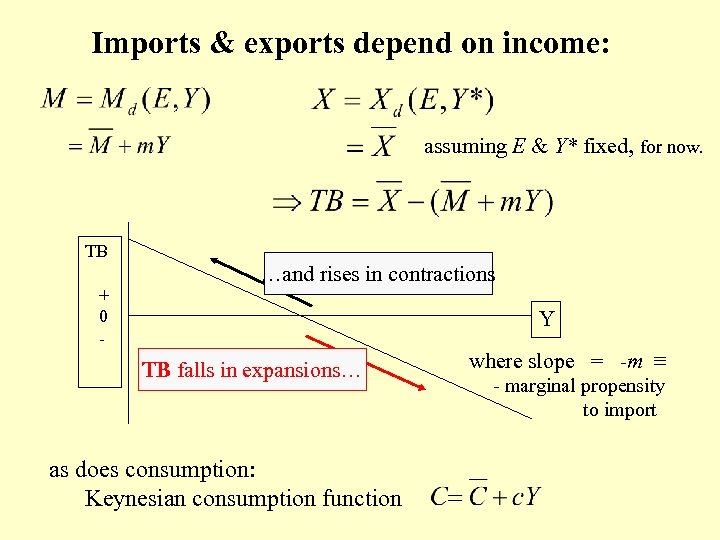Imports & exports depend on income: assuming E & Y* fixed, for now. TB + 0 - …and rises in contractions Y TB falls in expansions… as does consumption: Keynesian consumption function where slope = -m ≡ - marginal propensity to import

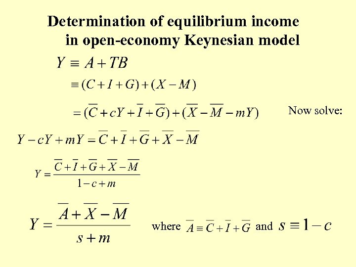Determination of equilibrium income in open-economy Keynesian model Now solve: where and

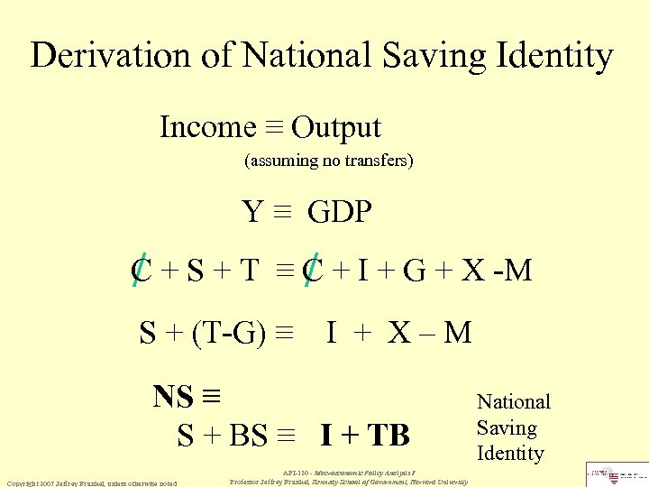Derivation of National Saving Identity Income ≡ Output (assuming no transfers) Y ≡ GDP C + S + T ≡ C + I + G + X -M / / S + (T-G) ≡ I + X–M NS ≡ S + BS ≡ I + TB Copyright 2007 Jeffrey Frankel, unless otherwise noted API-120 - Macroeconomic Policy Analysis I Professor Jeffrey Frankel, Kennedy School of Government, Harvard University National Saving Identity

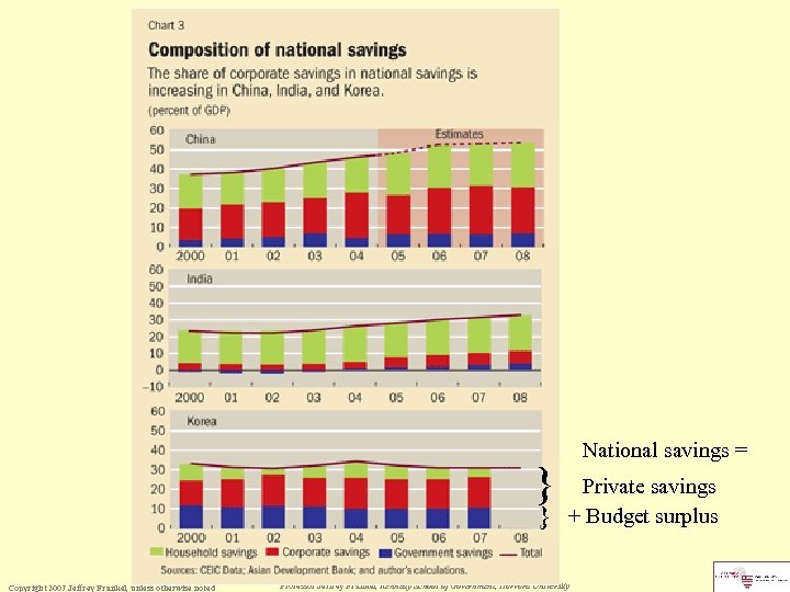} } Copyright 2007 Jeffrey Frankel, unless otherwise noted National savings = Private savings + Budget surplus API-120 - Macroeconomic Policy Analysis I Professor Jeffrey Frankel, Kennedy School of Government, Harvard University

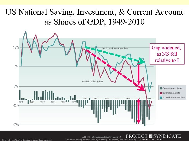US National Saving, Investment, & Current Account as Shares of GDP, 1949 -2010 Gap widened, as NS fell relative to I Copyright 2007 Jeffrey Frankel, unless otherwise noted API-120 - Macroeconomic Policy Analysis I Professor Jeffrey Frankel, Kennedy School of Government, Harvard University

Keynesian Consumption Function: or, expressed as a saving function: where s ≡ 1 – c } Copyright 2007 Jeffrey Frankel, unless otherwise noted API-120 - Macroeconomic Policy Analysis I Professor Jeffrey Frankel, Kennedy School of Government, Harvard University

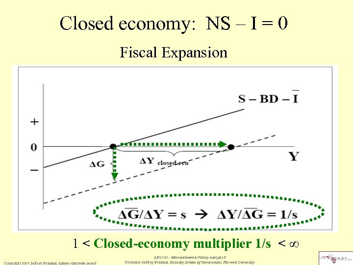Closed economy: NS – I = 0 Fiscal Expansion 1 < Closed-economy multiplier 1/s < ∞ Copyright 2007 Jeffrey Frankel, unless otherwise noted API-120 - Macroeconomic Policy Analysis I Professor Jeffrey Frankel, Kennedy School of Government, Harvard University

Open economy: NS – I = TB =X–M Imports: for simplicity Exports: for simplicity

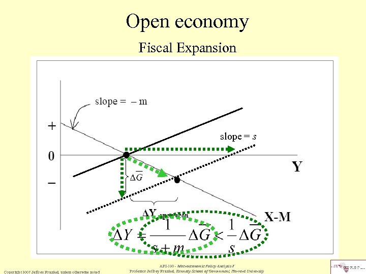Open economy Fiscal Expansion slope = s Copyright 2007 Jeffrey Frankel, unless otherwise noted API-120 - Macroeconomic Policy Analysis I Professor Jeffrey Frankel, Kennedy School of Government, Harvard University

Part 2: KEYNESIAN MULTIPLIERS • The multiplier for an increase in e. g. , due to a fiscal expansion. , • The multiplier for an increase in e. g. , due to a devaluation. , Copyright 2007 Jeffrey Frankel, unless otherwise noted API-120 - Macroeconomic Policy Analysis I Professor Jeffrey Frankel, Kennedy School of Government, Harvard University

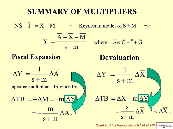SUMMARY OF MULTIPLIERS + Fiscal Expansion Keynesian model of S + M => Devaluation open-ec. multiplier = 1/(s+m)<1/s Equation (17. 11). Note misprint in 10 th ed. of WTP. )

Part 3: MACROECONOMIC INTERDEPENDENCE International transmission under fixed vs. floating exchange rates • of a disturbance originating domestically. • of a disturbance originating abroad. API-120 - Macroeconomic Policy Analysis I Professor Jeffrey Frankel, Kennedy School of Government, Harvard University

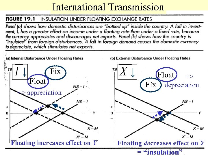International Transmission ↓ Fix Float => appreciation Floating increases effect on Y ↓ Float Fix => depreciation Floating decreases effect on Y = “insulation”

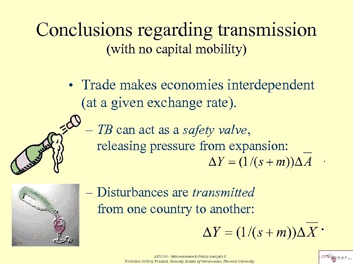Conclusions regarding transmission (with no capital mobility) • Trade makes economies interdependent (at a given exchange rate). – TB can act as a safety valve, releasing pressure from expansion: . – Disturbances are transmitted from one country to another: . API-120 - Macroeconomic Policy Analysis I Professor Jeffrey Frankel, Kennedy School of Government, Harvard University

Conclusions regarding transmission (with no capital mobility), continued • Floating exchange rates work to isolate effects of demand disturbances within the country where they originate: – Effects of a domestic disturbance tend to be “bottled up” within the country. In the extreme, floating reproduces the closed economy multiplier: . – The floating rate tends to insulate the domestic economy from effects of foreign disturbances. In the extreme, floating reproduces a closed economy: . API-120 - Macroeconomic Policy Analysis I Professor Jeffrey Frankel, Kennedy School of Government, Harvard University .

Parts 4 & 5: POLICY INSTRUMENTS Goals and Instruments • Policy goals: Internal balance & External balance • Policy instruments • The Swan Diagram • The principle of goals & instruments Introduction of monetary policy • The role of interest rates • Monetary expansion • Fiscal expansion & crowding out

Goals and instruments Policy Goals • Internal balance: Y = ≡ potential output ≡ ES ≡ “output gap” => unemployment > Y > ≡ ED => “overheating” => inflation e. g. , Y< and/or asset bubbles • External balance: e. g. , BP=0 or CA=0 Policy Instruments • Expenditure-reduction, e. g. , G ↓ • Expenditure-switching, e. g. , E ↑ Copyright 2007 Jeffrey Frankel, unless otherwise noted API-120 - Macroeconomic Policy Analysis I Professor Jeffrey Frankel, Kennedy School of Government, Harvard University

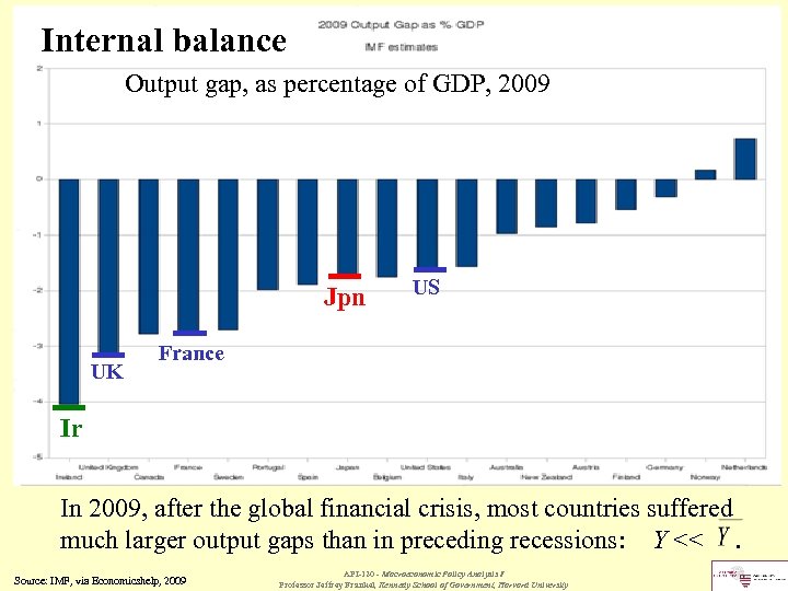Internal balance Output gap, as percentage of GDP, 2009 Jpn UK US France Ir In 2009, after the global financial crisis, most countries suffered much larger output gaps than in preceding recessions: Y <<. Source: IMF, via Economicshelp, 2009 Copyright 2007 Jeffrey Frankel, unless otherwise noted API-120 - Macroeconomic Policy Analysis I Professor Jeffrey Frankel, Kennedy School of Government, Harvard University

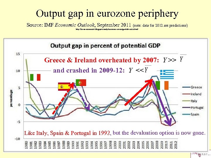Output gap in eurozone periphery Source: IMF Economic Outlook, September 2011 (note: data for 2012 are predictions) http: //im-an-economist. blogspot. com/p/eurozone-sovereign-debt-crisis. html Greece & Ireland overheated by 2007: Y >> and crashed in 2009 -12: Y << Like Italy, Spain & Portugal in 1992, but the devaluation option is now gone.

THE PRINCIPLE OF TARGETS AND INSTRUMENTS • Can’t normally hit 2 birds with 1 stone • Have n targets? • => Need n instruments, and they must be targeted independently. • Have 2 targets: CA = 0 and Y = ? • => Need 2 independent instruments: expenditure-reduction & expenditure-switching. Copyright 2007 Jeffrey Frankel, unless otherwise noted API-120 - Macroeconomic Policy Analysis I Professor Jeffrey Frankel, Kennedy School of Government, Harvard University

RESPONSES TO CURRENT ACCOUNT DEFICIT Financing • By borrowing • or running down reserves. vs. Adjustment • Expenditure-reduction (“belt-tightening”) • e. g. , fiscal or monetary contraction • or Expenditure-switching • e. g. , devaluation.

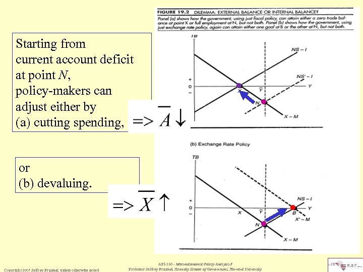Starting from current account deficit at point N, policy-makers can adjust either by (a) cutting spending, ● ● or (b) devaluing. ● ● Copyright 2007 Jeffrey Frankel, unless otherwise noted API-120 - Macroeconomic Policy Analysis I Professor Jeffrey Frankel, Kennedy School of Government, Harvard University

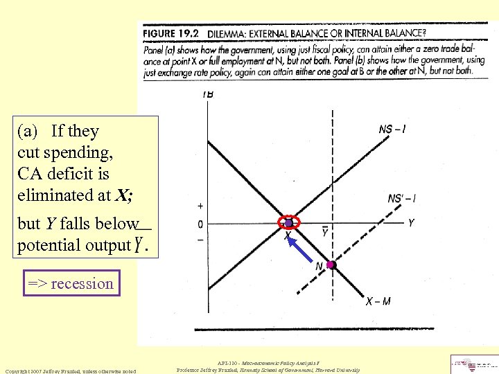(a) If they cut spending, CA deficit is eliminated at X; but Y falls below potential output. ● ● => recession Copyright 2007 Jeffrey Frankel, unless otherwise noted API-120 - Macroeconomic Policy Analysis I Professor Jeffrey Frankel, Kennedy School of Government, Harvard University

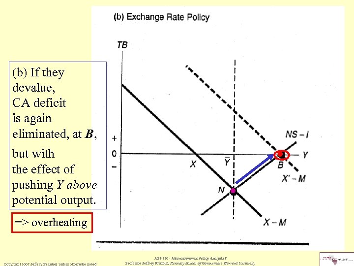(b) If they devalue, CA deficit is again eliminated, at B, but with the effect of pushing Y above potential output. ● ● => overheating Copyright 2007 Jeffrey Frankel, unless otherwise noted API-120 - Macroeconomic Policy Analysis I Professor Jeffrey Frankel, Kennedy School of Government, Harvard University

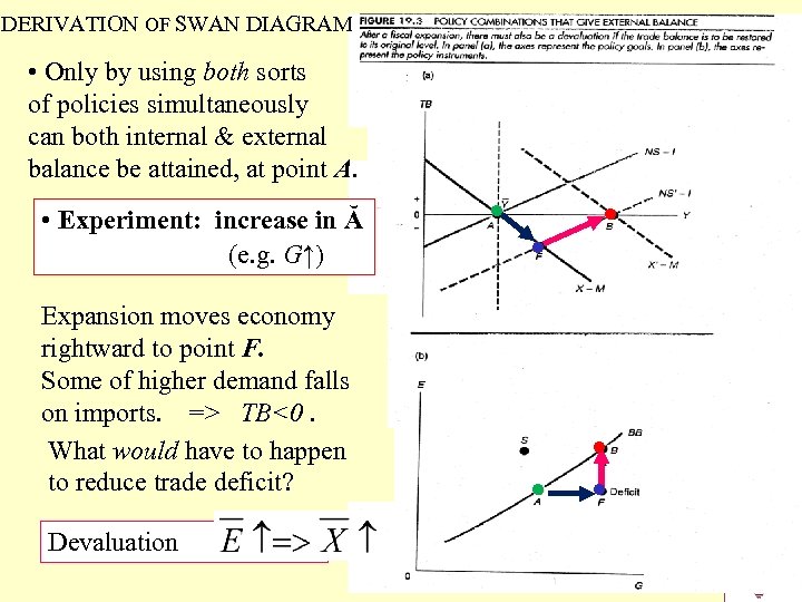DERIVATION OF SWAN DIAGRAM • Only by using both sorts of policies simultaneously can both internal & external balance be attained, at point A. • Experiment: increase in Ă (e. g. G↑) Expansion moves economy rightward to point F. Some of higher demand falls on imports. => TB<0. What would have to happen to reduce trade deficit? Devaluation ● ● ●

Again, At F, TB<0. What would have to happen to eliminate trade deficit? E↑. If depreciation is big enough, restores TB=0 at point B. ● ● ●

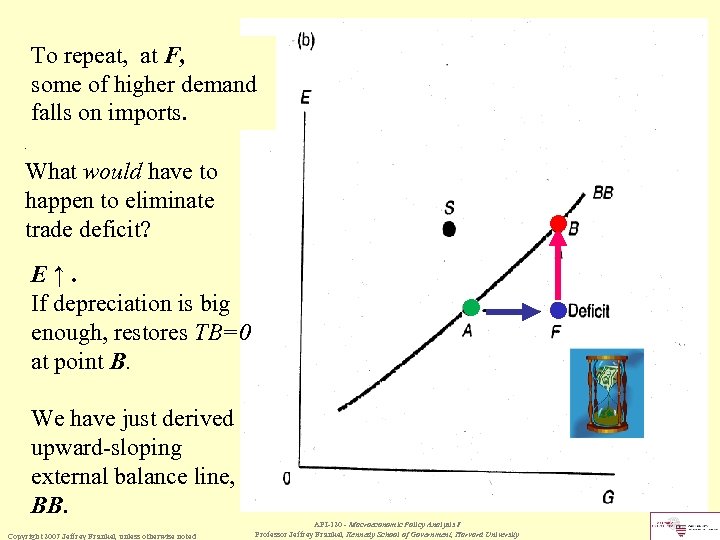To repeat, at F, some of higher demand falls on imports. . What would have to happen to eliminate trade deficit? E↑. If depreciation is big enough, restores TB=0 at point B. ● ● We have just derived upward-sloping external balance line, BB. Copyright 2007 Jeffrey Frankel, unless otherwise noted API-120 - Macroeconomic Policy Analysis I Professor Jeffrey Frankel, Kennedy School of Government, Harvard University ●

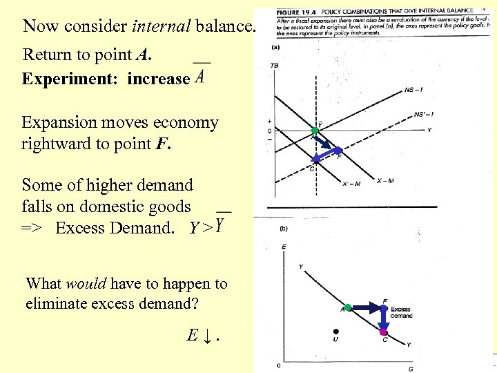Now consider internal balance. Return to point A. Experiment: increase Expansion moves economy rightward to point F. ● ● Some of higher demand falls on domestic goods => Excess Demand. Y > What would have to happen to eliminate excess demand? E↓. ● ● ●

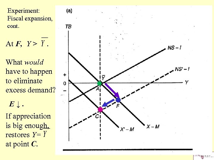Experiment: Fiscal expansion, cont. At F, Y > . What would have to happen to eliminate excess demand? E↓. If appreciation is big enough, restores Y= at point C. ● ● ●

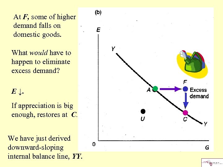At F, some of higher demand falls on domestic goods. What would have to happen to eliminate excess demand? E ↓. If appreciation is big enough, restores at C. We have just derived downward-sloping internal balance line, YY. ● ● ●

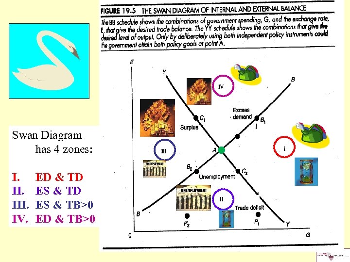Swan Diagram has 4 zones: I. III. IV. ED & TD ES & TB>0 ED & TB>0 ●

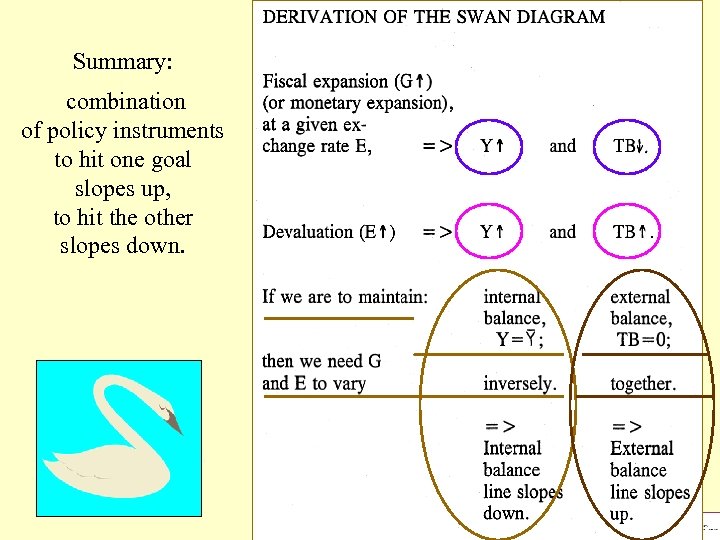Summary: combination of policy instruments to hit one goal slopes up, to hit the other slopes down.

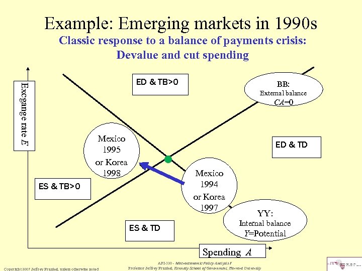Example: Emerging markets in 1990 s Classic response to a balance of payments crisis: Devalue and cut spending Excgange rate E ED & TB>0 BB: External balance CA=0 Mexico 1995 or Korea 1998 ED & TD ● Mexico 1994 or Korea 1997 ES & TB>0 ES & TD YY: Internal balance Y=Potential Spending A Copyright 2007 Jeffrey Frankel, unless otherwise noted API-120 - Macroeconomic Policy Analysis I Professor Jeffrey Frankel, Kennedy School of Government, Harvard University

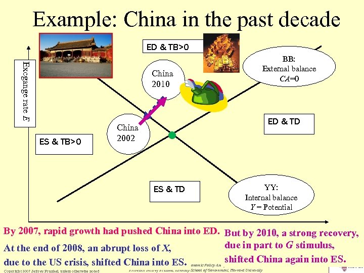Example: China in the past decade ED & TB>0 Excgange rate E China 2010 ES & TB>0 China 2002 BB: External balance CA=0 ED & TD ● ES & TD YY: Internal balance Y = Potential By 2007, rapid growth had pushed China into ED. But by 2010, a strong recovery, Spending A due in part to G stimulus, At the end of 2008, an abrupt loss of X, shifted China again into ES. due to the US crisis, shifted China into ES. Copyright 2007 Jeffrey Frankel, unless otherwise noted API-120 - Macroeconomic Policy Analysis I Professor Jeffrey Frankel, Kennedy School of Government, Harvard University

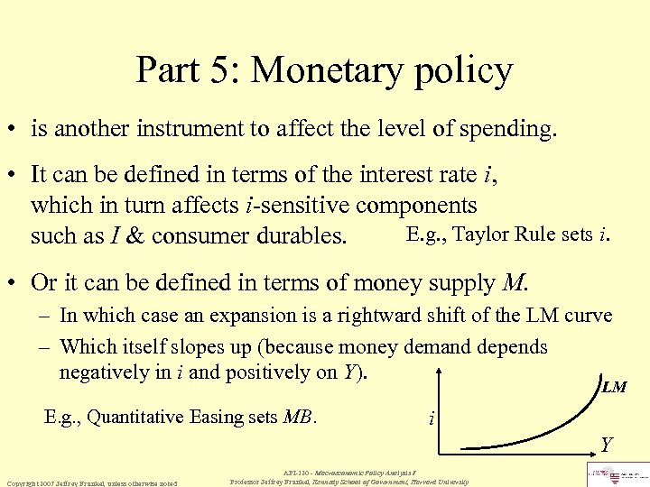Part 5: Monetary policy • is another instrument to affect the level of spending. • It can be defined in terms of the interest rate i, which in turn affects i-sensitive components E. g. , Taylor Rule sets i. such as I & consumer durables. • Or it can be defined in terms of money supply M. – In which case an expansion is a rightward shift of the LM curve – Which itself slopes up (because money demand depends negatively in i and positively on Y). LM E. g. , Quantitative Easing sets MB. i Y Copyright 2007 Jeffrey Frankel, unless otherwise noted API-120 - Macroeconomic Policy Analysis I Professor Jeffrey Frankel, Kennedy School of Government, Harvard University

Monetary expansion lowers i, stimulates demand, shifts NS-I down/out. New equilibrium at point M. In lower diagram, which shows i explicitly on the vertical axis, We’ve just derived IS curve. If monetary policy is defined by the level of money supply, then the same result is viewed as resulting from a rightward shift of the LM curve.

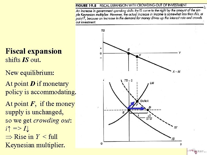Fiscal expansion shifts IS out. New equilibrium: At point D if monetary policy is accommodating. At point F, if the money supply is unchanged, so we get crowding out: i↑ => I↓ Þ Rise in Y < full Keynesian multiplier. . D

End of: Introduction to the Keynesian Model API-120 - Macroeconomic Policy Analysis, Prof. Jeffrey Frankel, Harvard Kennedy School