caa841517021a8a32eede6d4f471f117.ppt
- Количество слайдов: 164
 macro CHAPTER TEN Aggregate Demand I macroeconomics fifth edition N. Gregory Mankiw Power. Point® Slides by Ron Cronovich © 2004 Worth Publishers, all rights reserved
 The Big Picture Keynesian Cross Theory of Liquidity Preference IS curve LM curve IS-LM model Agg. demand curve Agg. supply curve CHAPTER 10 Aggregate Demand I Explanation of short-run fluctuations Model of Agg. Demand Agg. Supply 1
 Context § Chapter 9 introduced the model of aggregate demand aggregate supply. § Long run – prices flexible – output determined by factors of production & technology – unemployment equals its natural rate § Short run – prices fixed – output determined by aggregate demand – unemployment is negatively related to output CHAPTER 10 Aggregate Demand I 3
 Context § This chapter develops the IS-LM model, theory that yields the aggregate demand curve. § We focus on the short run and assume the price level is fixed. § This chapter (and chapter 11) focus on the closed-economy case. Chapter 12 presents the open-economy case. CHAPTER 10 Aggregate Demand I 4
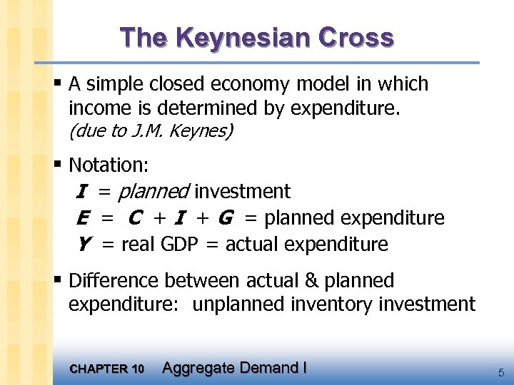 The Keynesian Cross § A simple closed economy model in which income is determined by expenditure. (due to J. M. Keynes) § Notation: I = planned investment E = C + I + G = planned expenditure Y = real GDP = actual expenditure § Difference between actual & planned expenditure: unplanned inventory investment CHAPTER 10 Aggregate Demand I 5
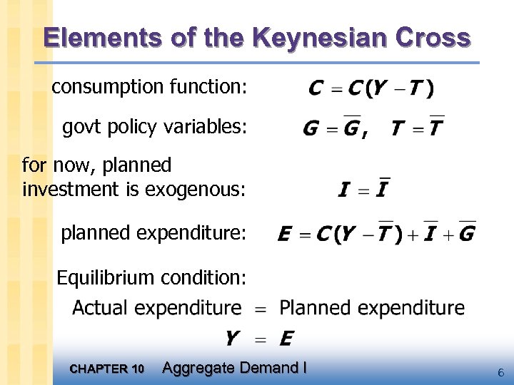 Elements of the Keynesian Cross consumption function: govt policy variables: for now, planned investment is exogenous: planned expenditure: Equilibrium condition: CHAPTER 10 Aggregate Demand I 6
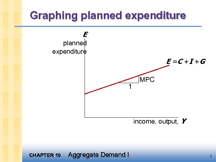 Graphing planned expenditure E = C +I +G 1 MPC income, output, Y CHAPTER 10 Aggregate Demand I 7
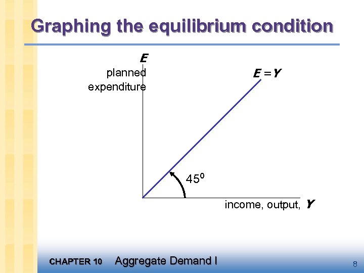 Graphing the equilibrium condition E E =Y planned expenditure 45º income, output, Y CHAPTER 10 Aggregate Demand I 8
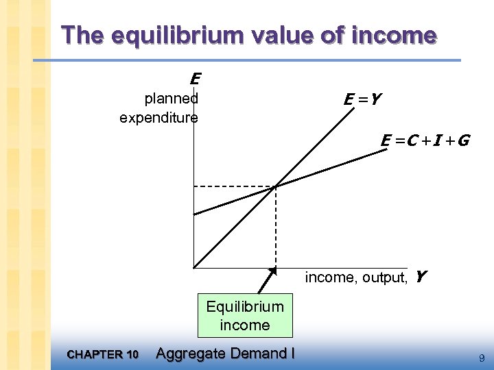 The equilibrium value of income E E =Y planned expenditure E = C +I +G income, output, Y Equilibrium income CHAPTER 10 Aggregate Demand I 9
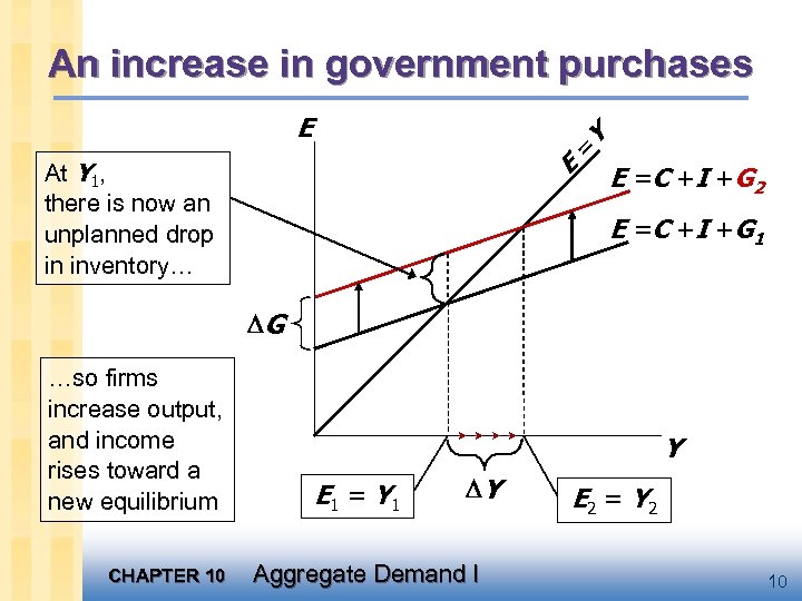 An increase in government purchases = E E At Y 1, there is now an unplanned drop in inventory… Y E = C + I + G 2 E = C + I + G 1 G …so firms increase output, and income rises toward a new equilibrium CHAPTER 10 Y E 1 = Y 1 Y Aggregate Demand I E 2 = Y 2 10
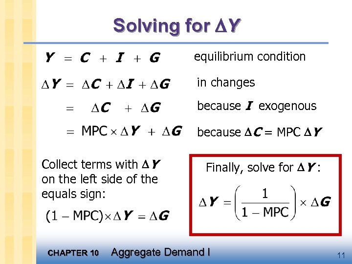 Solving for Y equilibrium condition in changes because I exogenous because C = MPC Y Collect terms with Y on the left side of the equals sign: CHAPTER 10 Finally, solve for Y : Aggregate Demand I 11
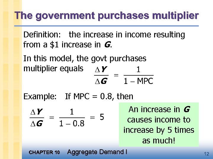 The government purchases multiplier Definition: the increase in income resulting from a $1 increase in G. In this model, the govt purchases multiplier equals Example: If MPC = 0. 8, then An increase in G causes income to increase by 5 times as much! CHAPTER 10 Aggregate Demand I 12
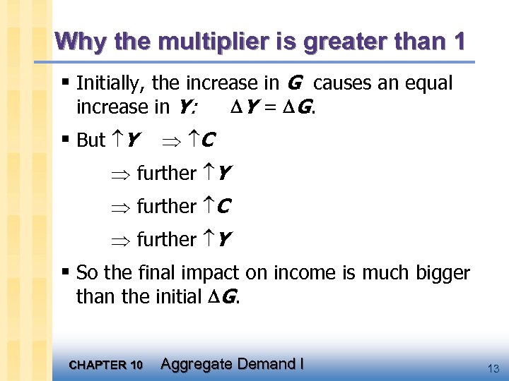 Why the multiplier is greater than 1 § Initially, the increase in G causes an equal increase in Y: § But Y Y = G. C further Y further C further Y § So the final impact on income is much bigger than the initial G. CHAPTER 10 Aggregate Demand I 13
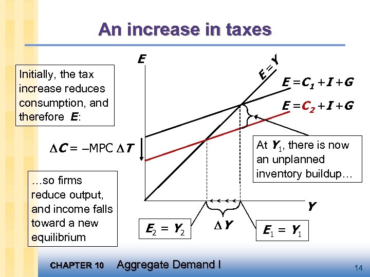 An increase in taxes = E Initially, the tax increase reduces consumption, and therefore E: E CHAPTER 10 E = C 1 +I +G E = C 2 +I +G At Y 1, there is now an unplanned inventory buildup… C = MPC T …so firms reduce output, and income falls toward a new equilibrium Y Y E 2 = Y 2 Y Aggregate Demand I E 1 = Y 1 14
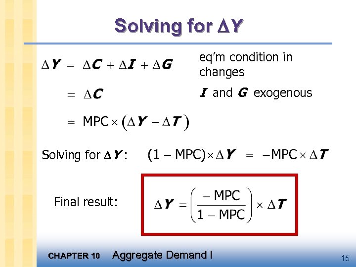 Solving for Y eq’m condition in changes I and G exogenous Solving for Y : Final result: CHAPTER 10 Aggregate Demand I 15
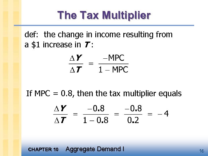 The Tax Multiplier def: the change in income resulting from a $1 increase in T : If MPC = 0. 8, then the tax multiplier equals CHAPTER 10 Aggregate Demand I 16
 The Tax Multiplier …is negative: A tax hike reduces consumer spending, which reduces income. …is greater than one (in absolute value): A change in taxes has a multiplier effect on income. …is smaller than the govt spending multiplier: Consumers save the fraction (1 -MPC) of a tax cut, so the initial boost in spending from a tax cut is smaller than from an equal increase in G. CHAPTER 10 Aggregate Demand I 17
 Exercise: § Use a graph of the Keynesian Cross to show the impact of an increase in planned investment on the equilibrium level of income/output. CHAPTER 10 Aggregate Demand I 18
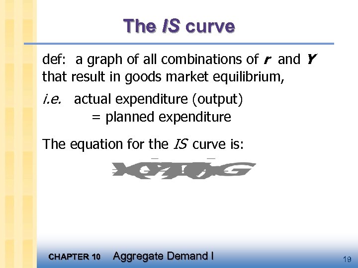 The IS curve def: a graph of all combinations of r and Y that result in goods market equilibrium, i. e. actual expenditure (output) = planned expenditure The equation for the IS curve is: CHAPTER 10 Aggregate Demand I 19
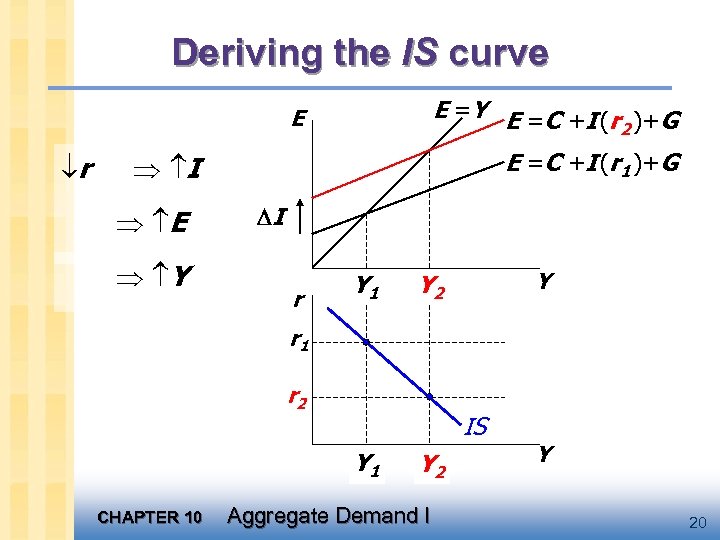 Deriving the IS curve E =Y E =C +I (r )+G 2 E r E =C +I (r 1 )+G I E Y I r Y 1 Y Y 2 r 1 r 2 IS Y 1 CHAPTER 10 Y 2 Aggregate Demand I Y 20
 Why the IS curve is negatively sloped § A fall in the interest rate motivates firms to increase investment spending, which drives up total planned spending (E ). § To restore equilibrium in the goods market, output (a. k. a. actual expenditure, Y ) must increase. CHAPTER 10 Aggregate Demand I 21
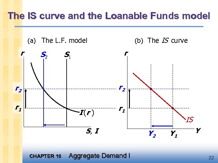 The IS curve and the Loanable Funds model (b) The IS curve (a) The L. F. model r S 2 r S 1 r 2 r 1 I (r ) S, I CHAPTER 10 Aggregate Demand I IS Y 2 Y 1 Y 22
 Fiscal Policy and the IS curve § We can use the IS-LM model to see how fiscal policy (G and T ) can affect aggregate demand output. § Let’s start by using the Keynesian Cross to see how fiscal policy shifts the IS curve… CHAPTER 10 Aggregate Demand I 23
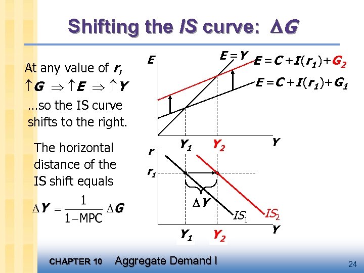 Shifting the IS curve: G At any value of r, G E Y …so the IS curve shifts to the right. The horizontal distance of the IS shift equals E =Y E =C +I (r )+G 1 2 E E =C +I (r 1 )+G 1 r Y 1 r 1 Y Y 1 CHAPTER 10 Y Y 2 IS 1 Y 2 Aggregate Demand I IS 2 Y 24
 Exercise: Shifting the IS curve § Use the diagram of the Keynesian Cross or Loanable Funds model to show an increase in taxes shifts the IS curve. CHAPTER 10 Aggregate Demand I 25
 The Theory of Liquidity Preference § due to John Maynard Keynes. § A simple theory in which the interest rate is determined by money supply and money demand. CHAPTER 10 Aggregate Demand I 26
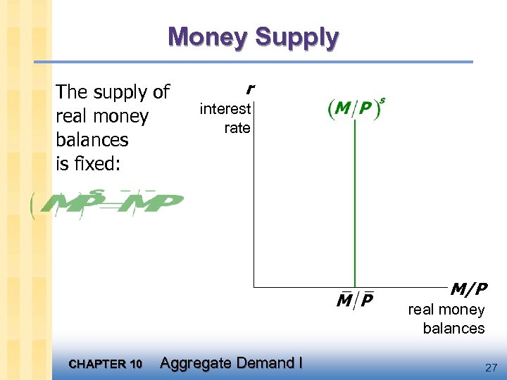 Money Supply The supply of real money balances is fixed: r interest rate M/P real money balances CHAPTER 10 Aggregate Demand I 27
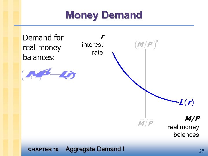 Money Demand for real money balances: r interest rate L (r ) M/P real money balances CHAPTER 10 Aggregate Demand I 28
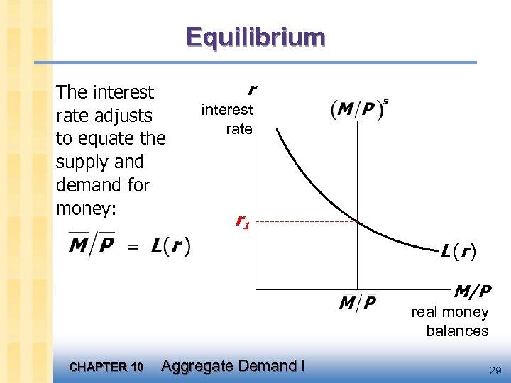 Equilibrium The interest rate adjusts to equate the supply and demand for money: r interest rate r 1 L (r ) M/P real money balances CHAPTER 10 Aggregate Demand I 29
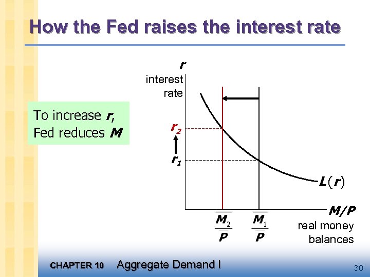 How the Fed raises the interest rate r interest rate To increase r, Fed reduces M r 2 r 1 L (r ) M/P real money balances CHAPTER 10 Aggregate Demand I 30
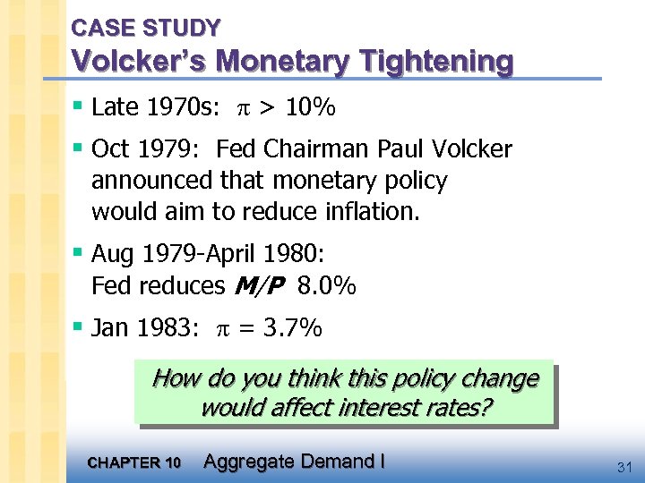 CASE STUDY Volcker’s Monetary Tightening § Late 1970 s: > 10% § Oct 1979: Fed Chairman Paul Volcker announced that monetary policy would aim to reduce inflation. § Aug 1979 -April 1980: Fed reduces M/P 8. 0% § Jan 1983: = 3. 7% How do you think this policy change would affect interest rates? CHAPTER 10 Aggregate Demand I 31
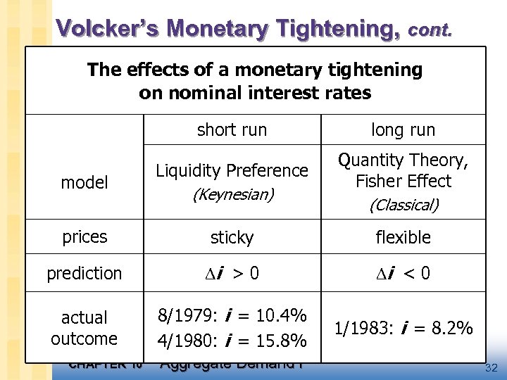 Volcker’s Monetary Tightening, cont. The effects of a monetary tightening on nominal interest rates short run model long run Liquidity Preference Quantity Theory, Fisher Effect (Keynesian) (Classical) prices sticky flexible prediction i > 0 i < 0 actual outcome 8/1979: i = 10. 4% 4/1980: i = 15. 8% 1/1983: i = 8. 2% CHAPTER 10 Aggregate Demand I 32
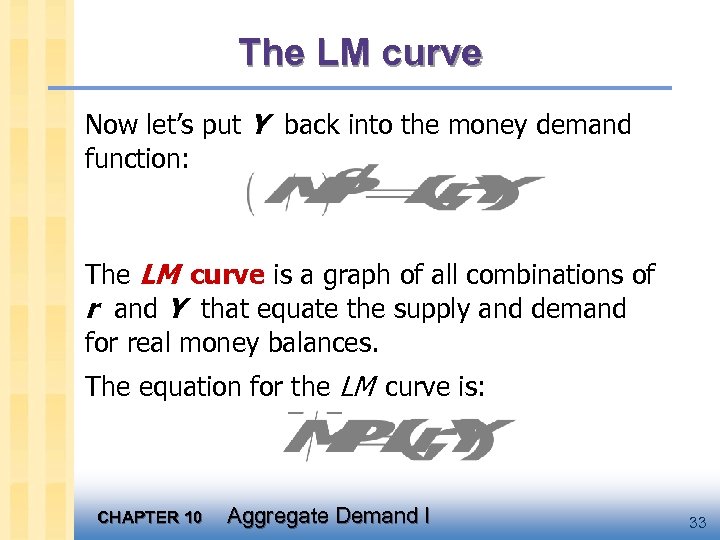 The LM curve Now let’s put Y back into the money demand function: The LM curve is a graph of all combinations of r and Y that equate the supply and demand for real money balances. The equation for the LM curve is: CHAPTER 10 Aggregate Demand I 33
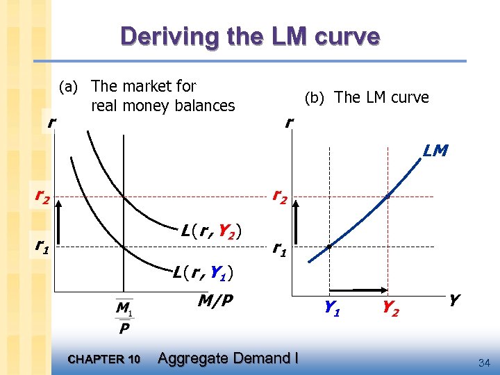 Deriving the LM curve (a) The market for r real money balances (b) The LM curve r LM r 2 L ( r , Y 2 ) r 1 L ( r , Y 1 ) M/P CHAPTER 10 Aggregate Demand I Y 1 Y 2 Y 34
 Why the LM curve is upward-sloping § An increase in income raises money demand. § Since the supply of real balances is fixed, there is now excess demand in the money market at the initial interest rate. § The interest rate must rise to restore equilibrium in the money market. CHAPTER 10 Aggregate Demand I 35
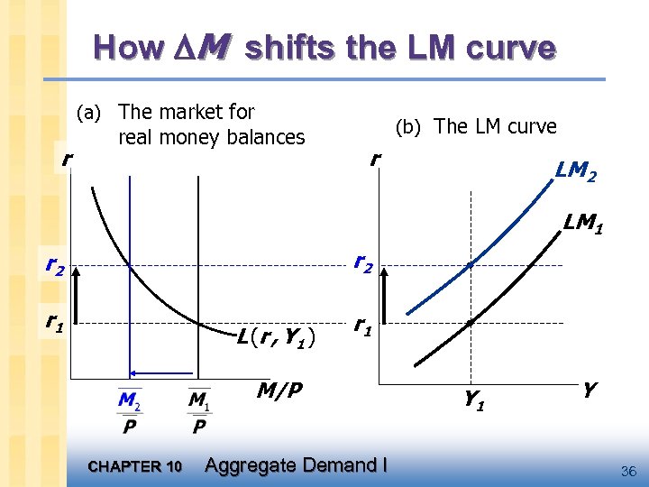 How M shifts the LM curve (a) The market for r real money balances (b) The LM curve r LM 2 LM 1 r 2 r 1 L ( r , Y 1 ) M/P CHAPTER 10 Aggregate Demand I Y 1 Y 36
 Exercise: Shifting the LM curve § Suppose a wave of credit card fraud causes consumers to use cash more frequently in transactions. § Use the Liquidity Preference model to show these events shift the LM curve. CHAPTER 10 Aggregate Demand I 37
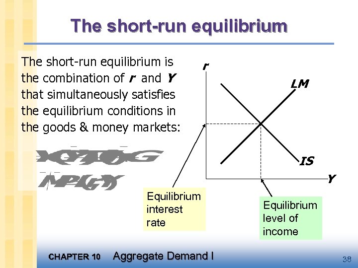 The short-run equilibrium is the combination of r and Y that simultaneously satisfies the equilibrium conditions in the goods & money markets: r LM IS Y Equilibrium interest rate CHAPTER 10 Aggregate Demand I Equilibrium level of income 38
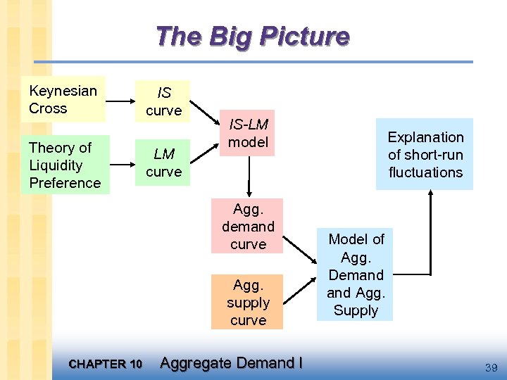 The Big Picture Keynesian Cross Theory of Liquidity Preference IS curve LM curve IS-LM model Agg. demand curve Agg. supply curve CHAPTER 10 Aggregate Demand I Explanation of short-run fluctuations Model of Agg. Demand Agg. Supply 39
 Chapter summary 1. Keynesian Cross § basic model of income determination § takes fiscal policy & investment as exogenous § fiscal policy has a multiplier effect on income. 2. IS curve § comes from Keynesian Cross when planned investment depends negatively on interest rate § shows all combinations of r and Y that equate planned expenditure with actual expenditure on goods & services CHAPTER 10 Aggregate Demand I 40
 Chapter summary 3. Theory of Liquidity Preference § basic model of interest rate determination § takes money supply & price level as exogenous § an increase in the money supply lowers the interest rate 4. LM curve § comes from Liquidity Preference Theory when money demand depends positively on income § shows all combinations of r and. Y that equate demand for real money balances with supply CHAPTER 10 Aggregate Demand I 41
 Chapter summary 5. IS-LM model § Intersection of IS and LM curves shows the unique point (Y, r ) that satisfies equilibrium in both the goods and money markets. CHAPTER 10 Aggregate Demand I 42
 Preview of Chapter 11 In Chapter 11, we will § use the IS-LM model to analyze the impact of policies and shocks § learn how the aggregate demand curve comes from IS-LM § use the IS-LM and AD-AS models together to analyze the short-run and long-run effects of shocks § use our models to learn about the Great Depression CHAPTER 10 Aggregate Demand I 43
 CHAPTER 10 Aggregate Demand I 44
 macro CHAPTER TEN Aggregate Demand I macroeconomics fifth edition N. Gregory Mankiw Power. Point® Slides by Ron Cronovich © 2004 Worth Publishers, all rights reserved
 Context § Chapter 9 introduced the model of aggregate demand supply. § Chapter 10 developed the IS-LM model, the basis of the aggregate demand curve. § In Chapter 11, we will use the IS-LM model to – see how policies and shocks affect income and the interest rate in the short run when prices are fixed – derive the aggregate demand curve – explore various explanations for the Great Depression CHAPTER 10 Aggregate Demand I 46
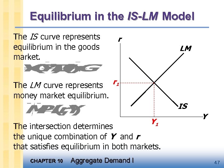 Equilibrium in the IS-LM Model The IS curve represents equilibrium in the goods market. r LM The LM curve represents r 1 money market equilibrium. IS Y 1 Y The intersection determines the unique combination of Y and r that satisfies equilibrium in both markets. CHAPTER 10 Aggregate Demand I 47
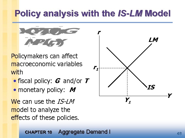 Policy analysis with the IS-LM Model r LM Policymakers can affect macroeconomic variables r 1 with • fiscal policy: G and/or T • monetary policy: M We can use the IS-LM model to analyze the effects of these policies. CHAPTER 10 Aggregate Demand I IS Y 1 Y 48
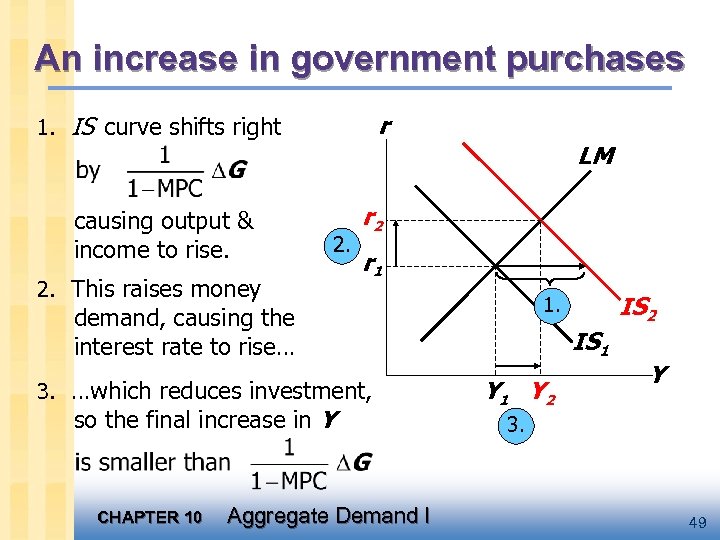 An increase in government purchases r 1. IS curve shifts right causing output & income to rise. 2. This raises money LM r 2 r 1 3. …which reduces investment, so the final increase in Y CHAPTER 10 Aggregate Demand I IS 2 1. demand, causing the interest rate to rise… IS 1 Y 2 Y 3. 49
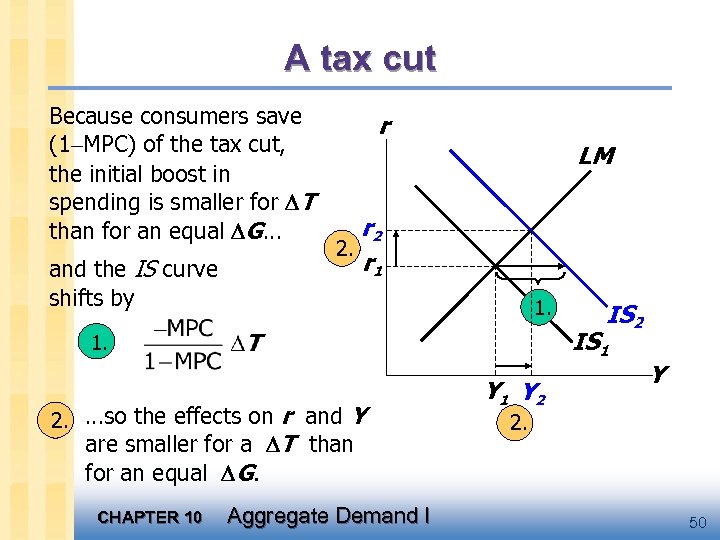 A tax cut Because consumers save (1 MPC) of the tax cut, the initial boost in spending is smaller for T than for an equal G… and the IS curve shifts by r LM r 2 2. r 1 1. IS 1 1. 2. …so the effects on r and Y are smaller for a T than for an equal G. CHAPTER 10 IS 2 Aggregate Demand I Y 1 Y 2. 50
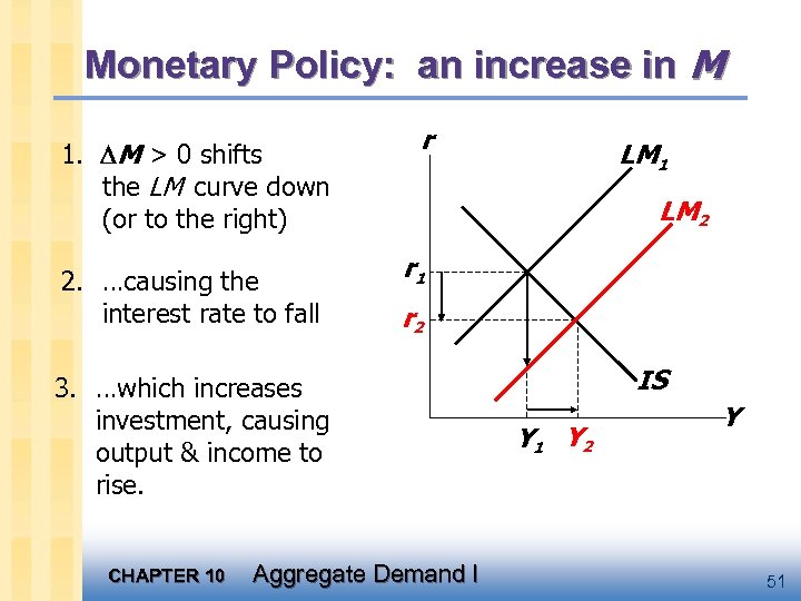 Monetary Policy: an increase in M 1. M > 0 shifts the LM curve down (or to the right) 2. …causing the interest rate to fall r LM 2 r 1 r 2 3. …which increases investment, causing output & income to rise. CHAPTER 10 LM 1 Aggregate Demand I IS Y 1 Y 2 Y 51
 Interaction between monetary & fiscal policy § Model: monetary & fiscal policy variables (M, G and T ) are exogenous § Real world: Monetary policymakers may adjust M in response to changes in fiscal policy, or vice versa. § Such interaction may alter the impact of the original policy change. CHAPTER 10 Aggregate Demand I 52
 The Fed’s response to G > 0 § Suppose Congress increases G. § Possible Fed responses: 1. hold M constant 2. hold r constant 3. hold Y constant § In each case, the effects of the G are different: CHAPTER 10 Aggregate Demand I 53
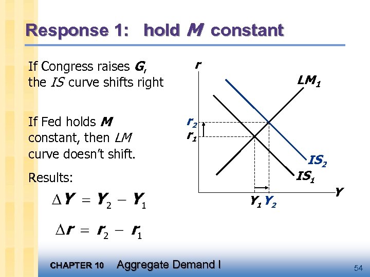 Response 1: hold M constant If Congress raises G, the IS curve shifts right If Fed holds M constant, then LM curve doesn’t shift. r LM 1 r 2 r 1 IS 2 IS 1 Results: Y 1 Y 2 CHAPTER 10 Aggregate Demand I Y 54
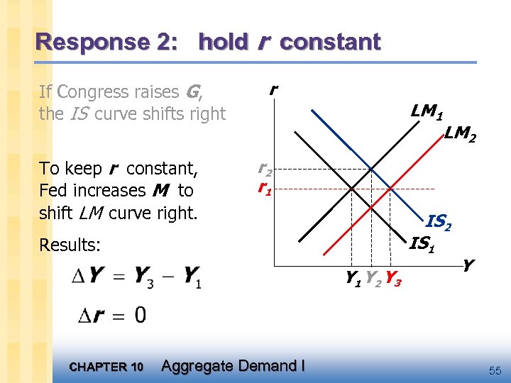 Response 2: hold r constant If Congress raises G, the IS curve shifts right To keep r constant, Fed increases M to shift LM curve right. r LM 1 r 2 r 1 IS 2 IS 1 Results: Y 1 Y 2 Y 3 CHAPTER 10 LM 2 Aggregate Demand I Y 55
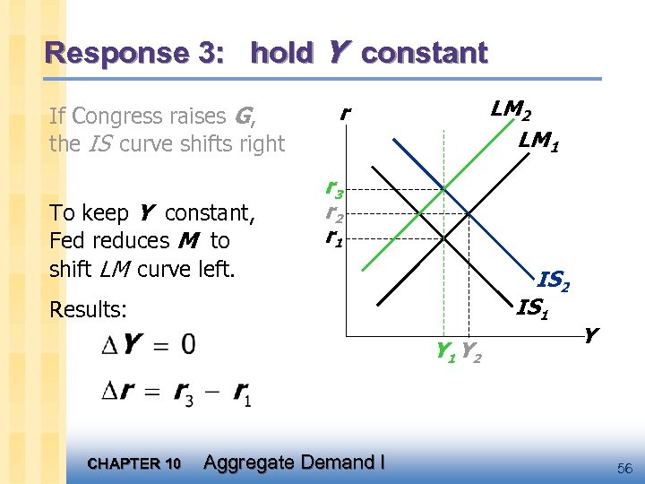 Response 3: hold Y constant If Congress raises G, the IS curve shifts right To keep Y constant, Fed reduces M to shift LM curve left. LM 2 LM 1 r r 3 r 2 r 1 IS 2 IS 1 Results: Y 1 Y 2 CHAPTER 10 Aggregate Demand I Y 56
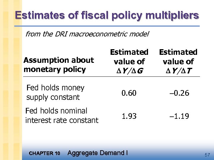 Estimates of fiscal policy multipliers from the DRI macroeconometric model Estimated value of Y / G Estimated value of Y / T Fed holds money supply constant 0. 60 0. 26 Fed holds nominal interest rate constant 1. 93 1. 19 Assumption about monetary policy CHAPTER 10 Aggregate Demand I 57
 Shocks in the IS-LM Model IS shocks: exogenous changes in the demand for goods & services. Examples: • stock market boom or crash change in households’ wealth C • change in business or consumer confidence or expectations I and/or C CHAPTER 10 Aggregate Demand I 58
 Shocks in the IS-LM Model LM shocks: exogenous changes in the demand for money. Examples: • a wave of credit card fraud increases demand for money • more ATMs or the Internet reduce money demand CHAPTER 10 Aggregate Demand I 59
 EXERCISE: Analyze shocks with the IS-LM model Use the IS-LM model to analyze the effects of 1. A boom in the stock market makes consumers wealthier. 2. After a wave of credit card fraud, consumers use cash more frequently in transactions. For each shock, a. use the IS-LM diagram to show the effects of the shock on Y and r. b. determine what happens to C, I, and the unemployment rate. CHAPTER 10 Aggregate Demand I 60
 CASE STUDY The U. S. economic slowdown of 2001 ~What happened~ 1. Real GDP growth rate 1994 -2000: 3. 9% (average annual) 2001: 0. 8% for the year, March 2001 determined to be the end of the longest expansion on record. 2. Unemployment rate Dec 2000: 3. 9% Dec 2001: 5. 8% The number of unemployed people rose by 2. 1 million during 2001! CHAPTER 10 Aggregate Demand I 61
 CASE STUDY The U. S. economic slowdown of 2001 ~Shocks that contributed to the slowdown~ 1. Falling stock prices From Aug 2000 to Aug 2001: -25% Week after 9/11: -12% 2. The terrorist attacks on 9/11 • increased uncertainty • fall in consumer & business confidence Both shocks reduced spending and shifted the IS curve left. CHAPTER 10 Aggregate Demand I 62
 CASE STUDY The U. S. economic slowdown of 2001 ~The policy response~ 1. Fiscal policy • large long-term tax cut, immediate $300 rebate checks • spending increases: aid to New York City & the airline industry, war on terrorism 2. Monetary policy • Fed lowered its Fed Funds rate target 11 times during 2001, from 6. 5% to 1. 75% • Money growth increased, interest rates fell CHAPTER 10 Aggregate Demand I 63
 CASE STUDY The U. S. economic slowdown of 2001 ~The recovery~ § The recession officially ended in November 2001. § Real GDP recovered, growing 2. 3% in 2002 and 4. 4% in 2003. § The unemployment rate lagged: 5. 8% in 2002, 6. 0% in 2003. § The Fed cut interest rates in 11/02 and 6/03. § Unemployment finally appears to be responding: 5. 6% for the first half of 2004. CHAPTER 10 Aggregate Demand I 64
 What is the Fed’s policy instrument? What the newspaper says: “the Fed lowered interest rates by one-half point today” What actually happened: The Fed conducted expansionary monetary policy to shift the LM curve to the right until the interest rate fell 0. 5 points. The Fed targets the Federal Funds rate: it announces a target value, and uses monetary policy to shift the LM curve as needed to attain its target rate. CHAPTER 10 Aggregate Demand I 65
 What is the Fed’s policy instrument? Why does the Fed target interest rates instead of the money supply? 1) They are easier to measure than the money supply 2) The Fed might believe that LM shocks are more prevalent than IS shocks. If so, then targeting the interest rate stabilizes income better than targeting the money supply. (See Problem 7 on p. 306) CHAPTER 10 Aggregate Demand I 66
 IS-LM and Aggregate Demand § So far, we’ve been using the IS-LM model to analyze the short run, when the price level is assumed fixed. § However, a change in P would shift the LM curve and therefore affect Y. § The aggregate demand curve (introduced in chap. 9 ) captures this relationship between P and Y CHAPTER 10 Aggregate Demand I 67
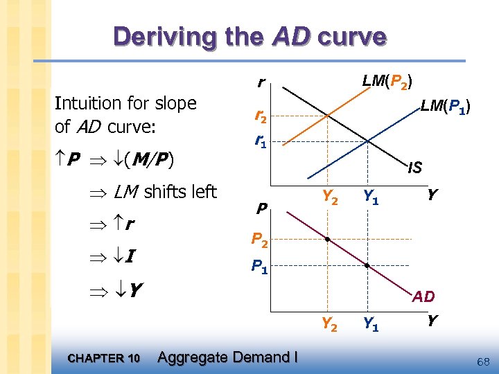 Deriving the AD curve r Intuition for slope of AD curve: P (M/P ) LM shifts left r I Y LM(P 2) LM(P 1) r 2 r 1 IS P Y 2 Y P 2 P 1 AD Y 2 CHAPTER 10 Y 1 Aggregate Demand I Y 1 Y 68
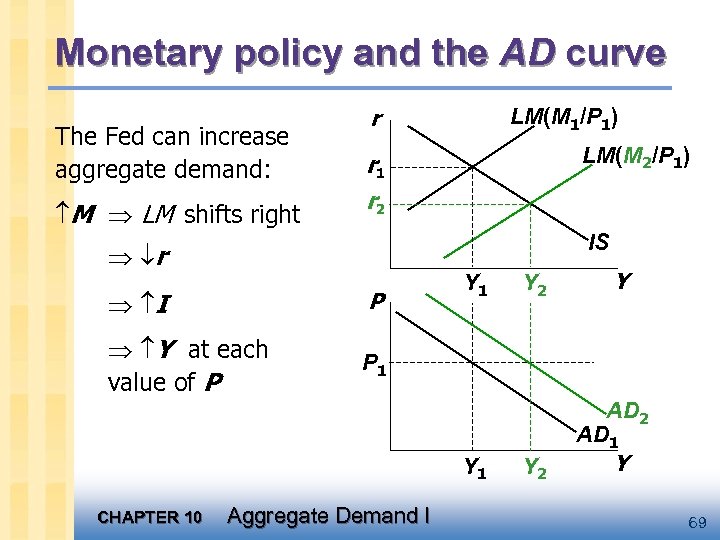 Monetary policy and the AD curve The Fed can increase aggregate demand: M LM shifts right r LM(M 1/P 1) LM(M 2/P 1) r 1 r 2 IS r I P Y at each value of P Y 1 Y 2 Y P 1 Y 1 CHAPTER 10 Aggregate Demand I Y 2 AD 1 Y 69
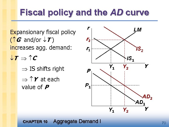 Fiscal policy and the AD curve Expansionary fiscal policy ( G and/or T ) increases agg. demand: r LM r 2 r 1 IS 2 T C IS 1 IS shifts right P Y at each value of P Y 1 Y 2 Y P 1 Y 1 CHAPTER 10 Aggregate Demand I Y 2 AD 1 Y 70
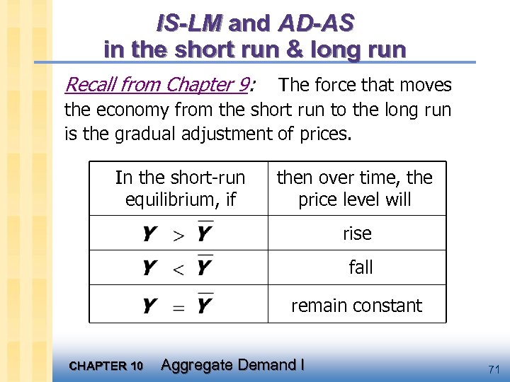 IS-LM and AD-AS in the short run & long run Recall from Chapter 9: The force that moves the economy from the short run to the long run is the gradual adjustment of prices. In the short-run equilibrium, if then over time, the price level will rise fall remain constant CHAPTER 10 Aggregate Demand I 71
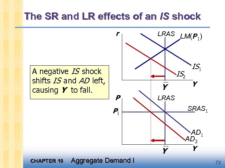 The SR and LR effects of an IS shock r A negative IS shock shifts IS and AD left, causing Y to fall. LRAS LM(P ) 1 IS 2 IS 1 Y P P 1 LRAS SRAS 1 AD 2 Y CHAPTER 10 Aggregate Demand I 72
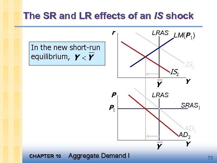 The SR and LR effects of an IS shock r LRAS LM(P ) 1 In the new short-run equilibrium, IS 2 IS 1 Y P P 1 LRAS SRAS 1 AD 2 Y CHAPTER 10 Aggregate Demand I 73
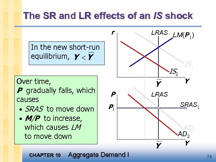 The SR and LR effects of an IS shock r LRAS LM(P ) 1 In the new short-run equilibrium, IS 2 Over time, P gradually falls, which causes • SRAS to move down • M/P to increase, which causes LM to move down CHAPTER 10 IS 1 Y P P 1 Aggregate Demand I LRAS SRAS 1 AD 2 Y 74
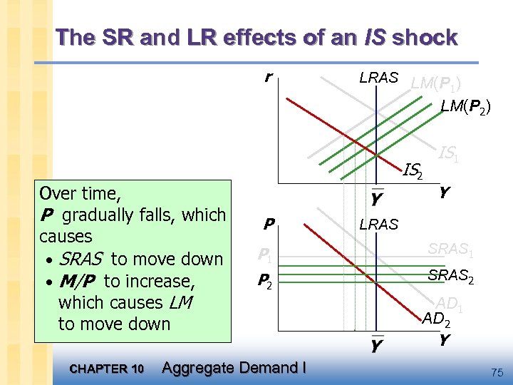 The SR and LR effects of an IS shock r LRAS LM(P ) 1 LM(P 2) IS 2 Over time, P gradually falls, which causes • SRAS to move down • M/P to increase, which causes LM to move down CHAPTER 10 IS 1 Y P LRAS P 1 SRAS 1 P 2 SRAS 2 Aggregate Demand I AD 1 AD 2 Y 75
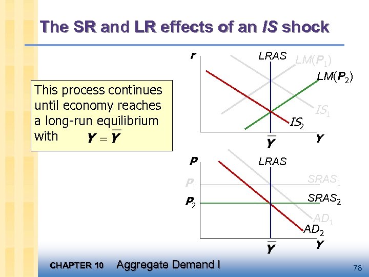 The SR and LR effects of an IS shock r LRAS LM(P ) 1 LM(P 2) This process continues until economy reaches a long-run equilibrium with IS 2 IS 1 Y P LRAS P 1 SRAS 1 P 2 SRAS 2 AD 1 AD 2 Y CHAPTER 10 Aggregate Demand I 76
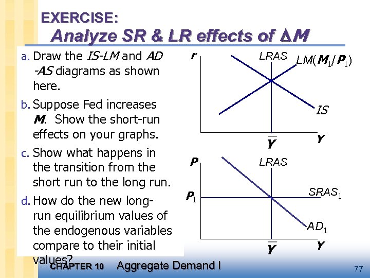 EXERCISE: Analyze SR & LR effects of M a. Draw the IS-LM and AD r -AS diagrams as shown here. b. Suppose Fed increases M. Show the short-run effects on your graphs. c. Show what happens in the transition from the short run to the long run. d. How do the new long- LRAS LM(M /P ) 1 1 IS Y P P 1 run equilibrium values of the endogenous variables compare to their initial values? CHAPTER 10 Aggregate Demand I LRAS SRAS 1 AD 1 Y 77
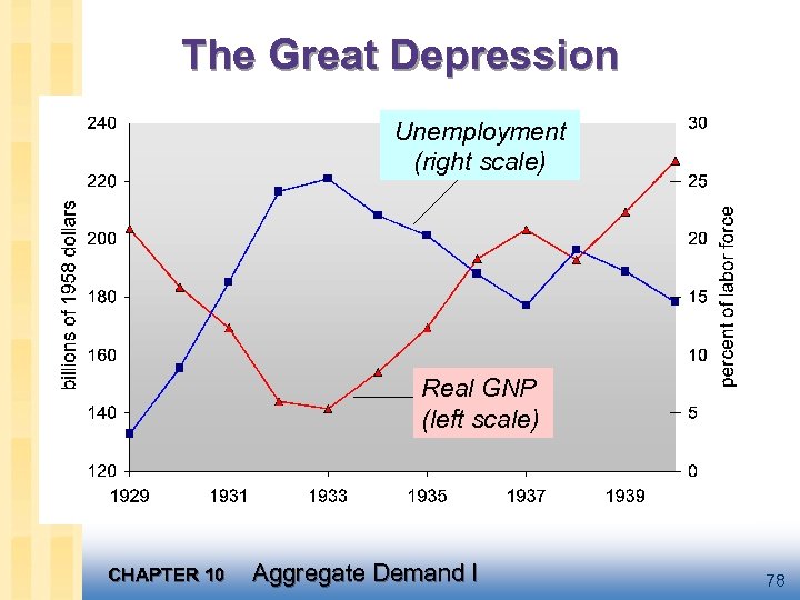 The Great Depression Unemployment (right scale) Real GNP (left scale) CHAPTER 10 Aggregate Demand I 78
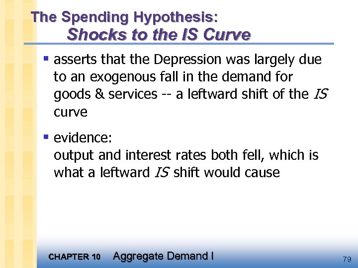 The Spending Hypothesis: Shocks to the IS Curve § asserts that the Depression was largely due to an exogenous fall in the demand for goods & services -- a leftward shift of the IS curve § evidence: output and interest rates both fell, which is what a leftward IS shift would cause CHAPTER 10 Aggregate Demand I 79
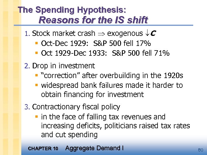 The Spending Hypothesis: Reasons for the IS shift 1. Stock market crash exogenous C § Oct-Dec 1929: S&P 500 fell 17% § Oct 1929 -Dec 1933: S&P 500 fell 71% 2. Drop in investment § “correction” after overbuilding in the 1920 s § widespread bank failures made it harder to obtain financing for investment 3. Contractionary fiscal policy § in the face of falling tax revenues and increasing deficits, politicians raised tax rates and cut spending CHAPTER 10 Aggregate Demand I 80
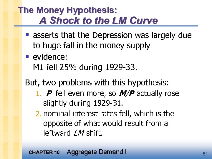 The Money Hypothesis: A Shock to the LM Curve § asserts that the Depression was largely due to huge fall in the money supply § evidence: M 1 fell 25% during 1929 -33. But, two problems with this hypothesis: 1. P fell even more, so M/P actually rose slightly during 1929 -31. 2. nominal interest rates fell, which is the opposite of what would result from a leftward LM shift. CHAPTER 10 Aggregate Demand I 81
 The Money Hypothesis Again: The Effects of Falling Prices § asserts that the severity of the Depression was due to a huge deflation: P fell 25% during 1929 -33. § This deflation was probably caused by the fall in M, so perhaps money played an important role after all. § In what ways does a deflation affect the economy? CHAPTER 10 Aggregate Demand I 82
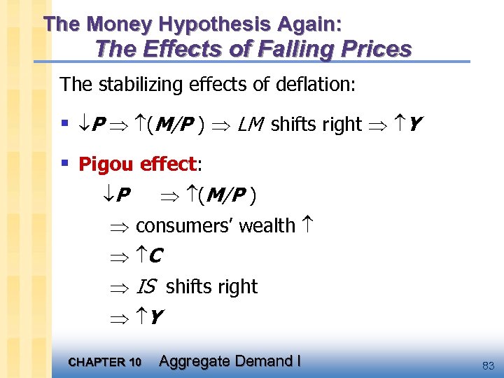 The Money Hypothesis Again: The Effects of Falling Prices The stabilizing effects of deflation: § P (M/P ) LM shifts right Y § Pigou effect: P (M/P ) consumers’ wealth C IS shifts right Y CHAPTER 10 Aggregate Demand I 83
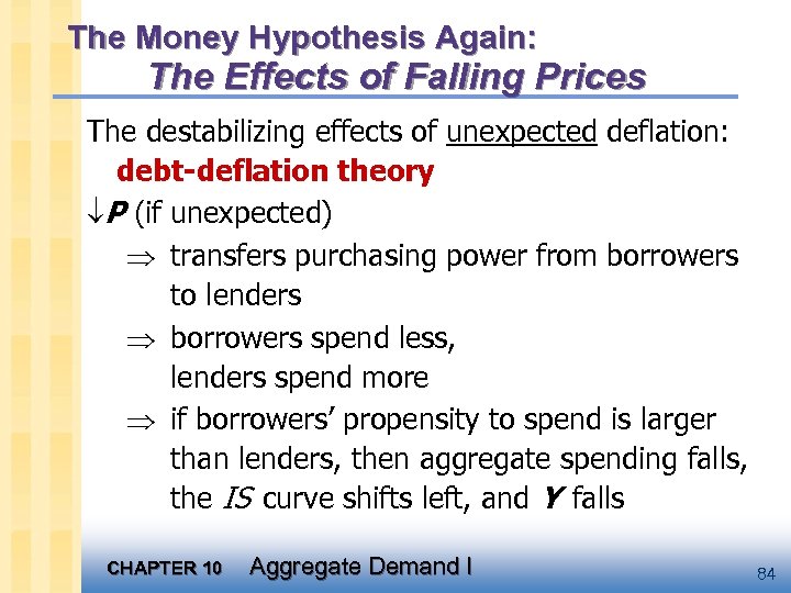 The Money Hypothesis Again: The Effects of Falling Prices The destabilizing effects of unexpected deflation: debt-deflation theory P (if unexpected) transfers purchasing power from borrowers to lenders borrowers spend less, lenders spend more if borrowers’ propensity to spend is larger than lenders, then aggregate spending falls, the IS curve shifts left, and Y falls CHAPTER 10 Aggregate Demand I 84
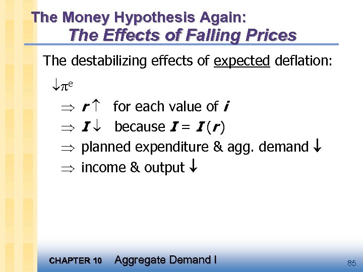 The Money Hypothesis Again: The Effects of Falling Prices The destabilizing effects of expected deflation: e r for each value of i I because I = I (r ) planned expenditure & agg. demand income & output CHAPTER 10 Aggregate Demand I 85
 Why another Depression is unlikely § Policymakers (or their advisors) now know much more about macroeconomics: § The Fed knows better than to let M fall so much, especially during a contraction. § Fiscal policymakers know better than to raise taxes or cut spending during a contraction. § Federal deposit insurance makes widespread bank failures very unlikely. § Automatic stabilizers make fiscal policy expansionary during an economic downturn. CHAPTER 10 Aggregate Demand I 86
 Chapter summary 1. IS-LM model § a theory of aggregate demand § exogenous: M, G, T, P exogenous in short run, Y in long run § endogenous: r, Y endogenous in short run, P in long run § IS curve: goods market equilibrium § LM curve: money market equilibrium CHAPTER 10 Aggregate Demand I 87
 Chapter summary 2. AD curve § shows relation between P and the IS-LM model’s equilibrium Y. § negative slope because P (M/P ) r I Y § expansionary fiscal policy shifts IS curve right, raises income, and shifts AD curve right § expansionary monetary policy shifts LM curve right, raises income, and shifts AD curve right § IS or LM shocks shift the AD curve CHAPTER 10 Aggregate Demand I 88
 CHAPTER 10 Aggregate Demand I 89
 macro CHAPTER TWELVE CHAPTER TEN Aggregate Demand I Aggregate Demand in the Open Economy macroeconomics fifth edition N. Gregory Mankiw Power. Point® Slides by Ron Cronovich © 2004 Worth Publishers, all rights reserved
 Learning objectives § The Mundell-Fleming model: IS-LM for the small open economy § Causes and effects of interest rate differentials § Arguments for fixed vs. floating exchange rates § The aggregate demand curve for the small open economy CHAPTER 10 Aggregate Demand I 91
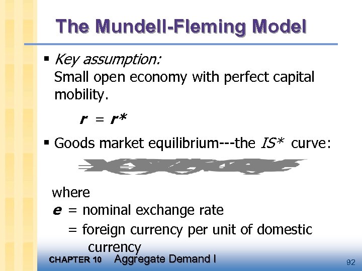 The Mundell-Fleming Model § Key assumption: Small open economy with perfect capital mobility. r = r* § Goods market equilibrium---the IS* curve: where e = nominal exchange rate = foreign currency per unit of domestic currency CHAPTER 10 Aggregate Demand I 92
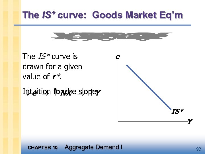 The IS* curve: Goods Market Eq’m The IS* curve is drawn for a given value of r*. e Intuition for the slope: IS* Y CHAPTER 10 Aggregate Demand I 93
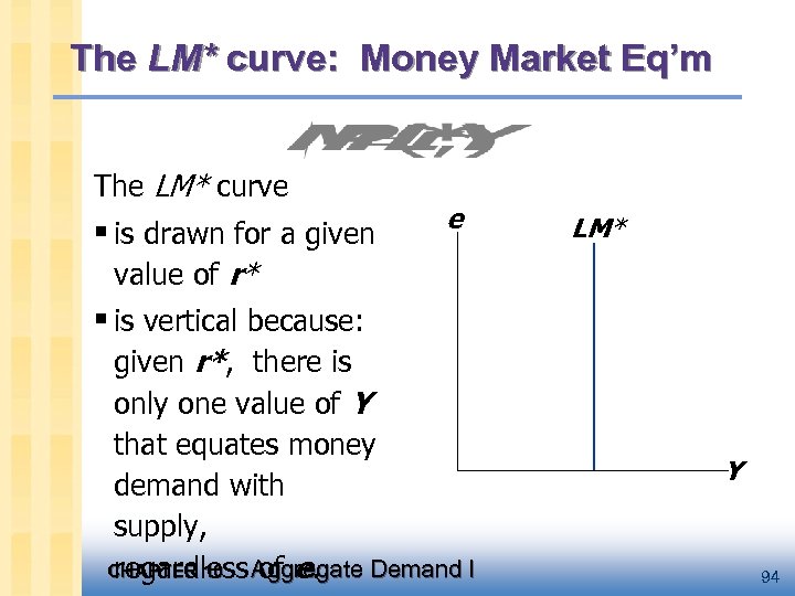 The LM* curve: Money Market Eq’m The LM* curve § is drawn for a given e LM* value of r* § is vertical because: given r*, there is only one value of Y that equates money demand with supply, CHAPTER 10 Aggregate Demand I regardless of e. Y 94
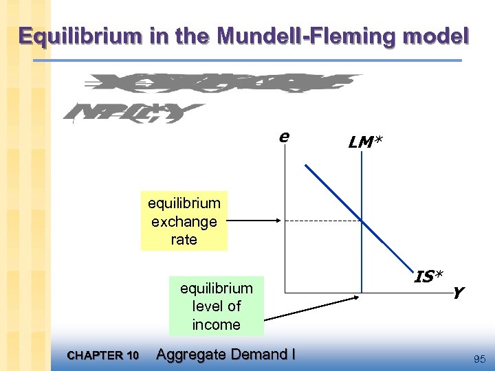 Equilibrium in the Mundell-Fleming model e LM* equilibrium exchange rate equilibrium level of income CHAPTER 10 Aggregate Demand I IS* Y 95
 Floating & fixed exchange rates § In a system of floating exchange rates, e is allowed to fluctuate in response to changing economic conditions. § In contrast, under fixed exchange rates, the central bank trades domestic foreign currency at a predetermined price. § We now consider fiscal, monetary, and trade policy: first in a floating exchange rate system, then in a fixed exchange rate system. CHAPTER 10 Aggregate Demand I 96
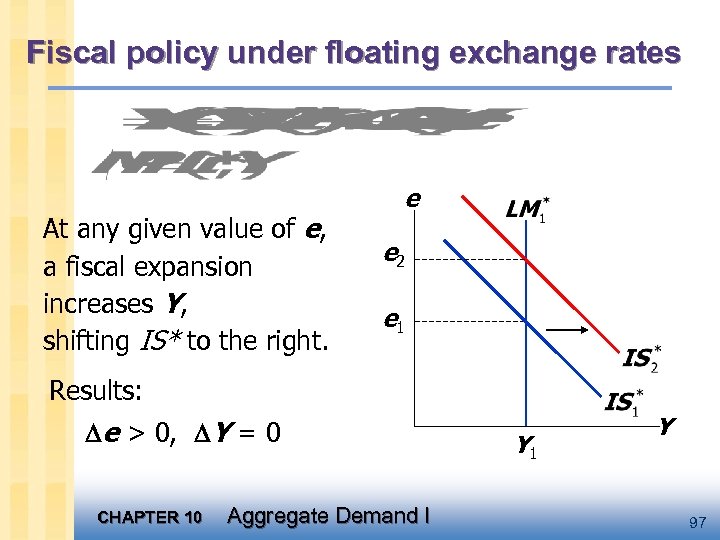 Fiscal policy under floating exchange rates At any given value of e, a fiscal expansion increases Y, shifting IS* to the right. e e 2 e 1 Results: e > 0, Y = 0 CHAPTER 10 Aggregate Demand I Y 1 Y 97
 Lessons about fiscal policy § In a small open economy with perfect capital mobility, fiscal policy cannot affect real GDP. § “Crowding out” • closed economy: Fiscal policy crowds out investment by causing the interest rate to rise. • small open economy: Fiscal policy crowds out net exports by causing the exchange rate to appreciate. CHAPTER 10 Aggregate Demand I 98
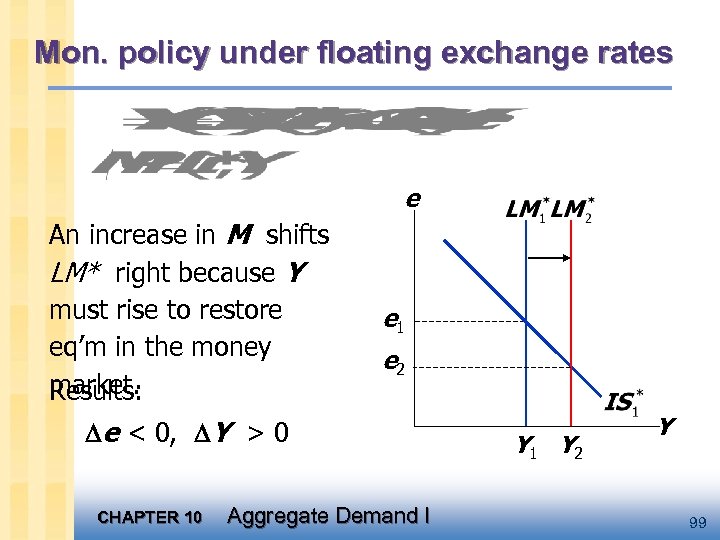 Mon. policy under floating exchange rates e An increase in M shifts LM* right because Y must rise to restore eq’m in the money market. Results: e 1 e 2 e < 0, Y > 0 CHAPTER 10 Aggregate Demand I Y 1 Y 2 Y 99
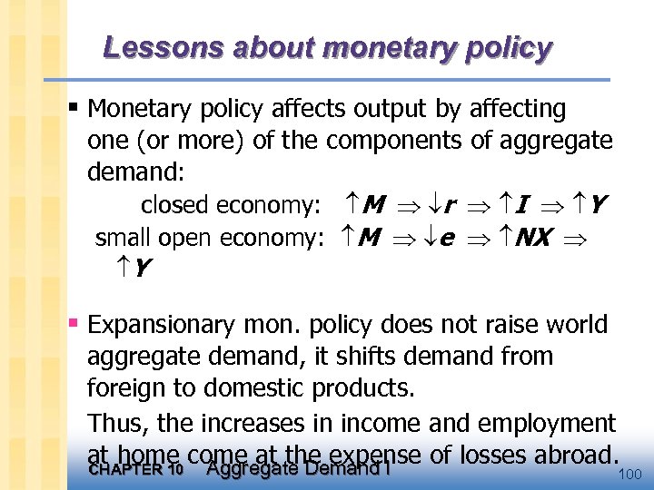 Lessons about monetary policy § Monetary policy affects output by affecting one (or more) of the components of aggregate demand: closed economy: M r I Y small open economy: M e NX Y § Expansionary mon. policy does not raise world aggregate demand, it shifts demand from foreign to domestic products. Thus, the increases in income and employment at home come at the expense of losses abroad. CHAPTER 10 Aggregate Demand I 100
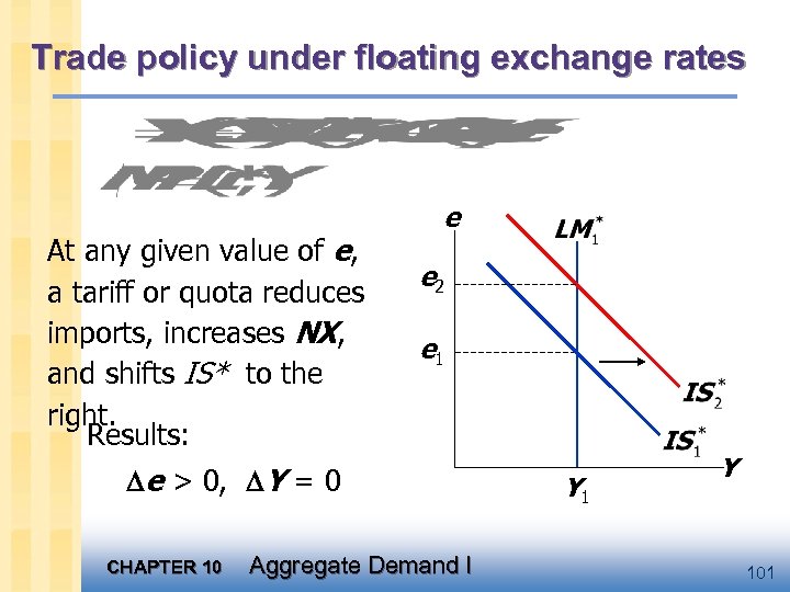 Trade policy under floating exchange rates At any given value of e, a tariff or quota reduces imports, increases NX, and shifts IS* to the right. Results: e e 2 e 1 e > 0, Y = 0 CHAPTER 10 Aggregate Demand I Y 101
 Lessons about trade policy § Import restrictions cannot reduce a trade deficit. § Even though NX is unchanged, there is less trade: – the trade restriction reduces imports – the exchange rate appreciation reduces exports Less trade means fewer ‘gains from trade. ’ § Import restrictions on specific products save jobs in the domestic industries that produce those products, but destroy jobs in export-producing sectors. Hence, import restrictions fail to increase total employment. CHAPTER 10 Aggregate Demand I Worse yet, import restrictions create “sectoral 102
 Fixed exchange rates § Under a system of fixed exchange rates, the country’s central bank stands ready to buy or sell the domestic currency foreign currency at a predetermined rate. § In the context of the Mundell-Fleming model, the central bank shifts the LM* curve as required to keep e at its preannounced rate. § This system fixes the nominal exchange rate. In the long run, when prices are flexible, the real exchange rate can move even if the nominal rate is fixed. CHAPTER 10 Aggregate Demand I 103
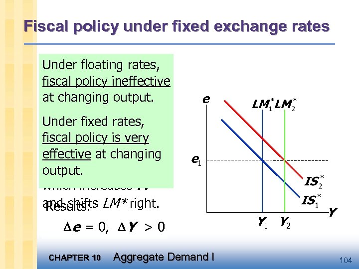 Fiscal policy under fixed exchange rates Under floating rates, a fiscal expansion would policy ineffective at changing output. raise e. To keep e from rising, Under fixed rates, the central bank must fiscal policy is very sell domestic effective at changing currency, output. which increases M and shifts LM* right. Results: e e 1 e = 0, Y > 0 CHAPTER 10 Aggregate Demand I Y 1 Y 2 Y 104
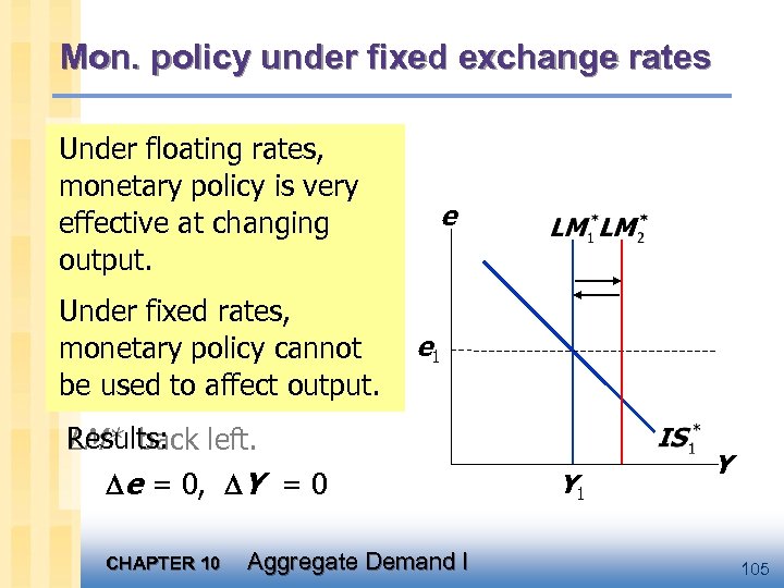 Mon. policy under fixed exchange rates An increase in M would Under floating rates, shift LM* right andvery monetary policy is reduce e effective at the fall in e. To prevent changing. output. e, the central bank Under buy domestic must fixed rates, e 1 monetary policy cannot currency, which be used to affectshifts reduces M and output. Results: LM* back left. e = 0, Y = 0 CHAPTER 10 Aggregate Demand I Y 105
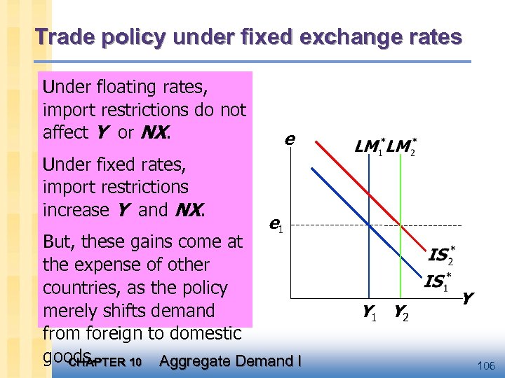 Trade policy under fixed exchange rates Under floating on A restriction rates, import restrictions do not imports puts upward affect Y oron e. pressure NX. e To keep e from Under fixed rates, rising, import restrictions must the central bank increase Y and NX. sell domestic e 1 currency, But, these gains come at which increases M the expense of other countries, as. LM* policy and shifts the right. Results: merely e = 0, demand 0 shifts Y > from foreign to domestic goods. CHAPTER 10 Aggregate Demand I Y 1 Y 2 Y 106
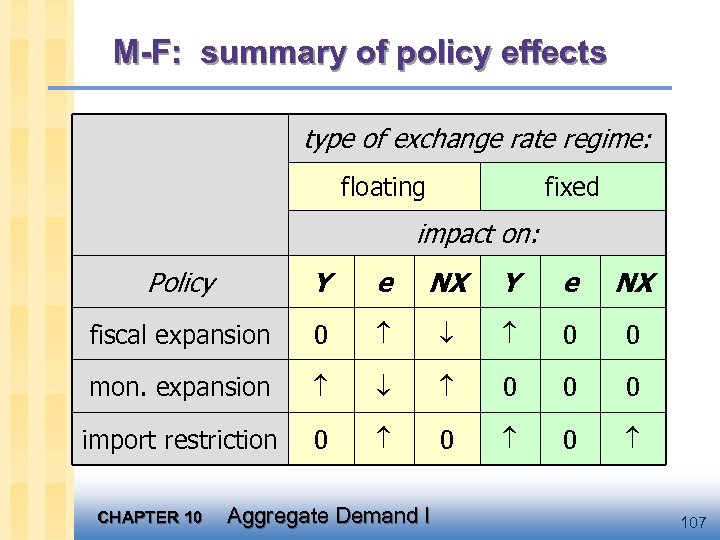 M-F: summary of policy effects type of exchange rate regime: floating fixed impact on: Policy Y e NX fiscal expansion 0 0 0 mon. expansion 0 0 0 import restriction 0 0 0 CHAPTER 10 Aggregate Demand I 107
 Interest-rate differentials Two reasons why r may differ from r* § country risk: The risk that the country’s borrowers will default on their loan repayments because of political or economic turmoil. Lenders require a higher interest rate to compensate them for this risk. § expected exchange rate changes: If a country’s exchange rate is expected to fall, then its borrowers must pay a higher interest rate to compensate lenders for the expected currency depreciation. CHAPTER 10 Aggregate Demand I 108
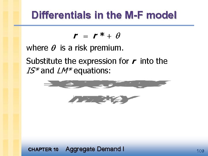 Differentials in the M-F model where is a risk premium. Substitute the expression for r into the IS* and LM* equations: CHAPTER 10 Aggregate Demand I 109
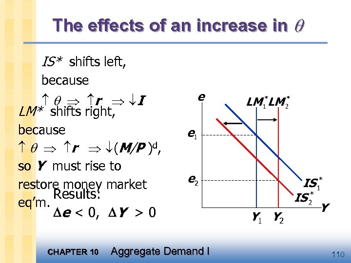 The effects of an increase in IS* shifts left, because r I LM* shifts right, because r (M/P )d, so Y must rise to restore money market Results: eq’m. e < 0, Y > 0 CHAPTER 10 e e 1 e 2 Aggregate Demand I Y 1 Y 2 Y 110
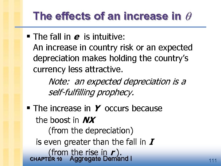 The effects of an increase in § The fall in e is intuitive: An increase in country risk or an expected depreciation makes holding the country’s currency less attractive. Note: an expected depreciation is a self-fulfilling prophecy. § The increase in Y occurs because the boost in NX (from the depreciation) is even greater than the fall in I (from the rise in r ). CHAPTER 10 Aggregate Demand I 111
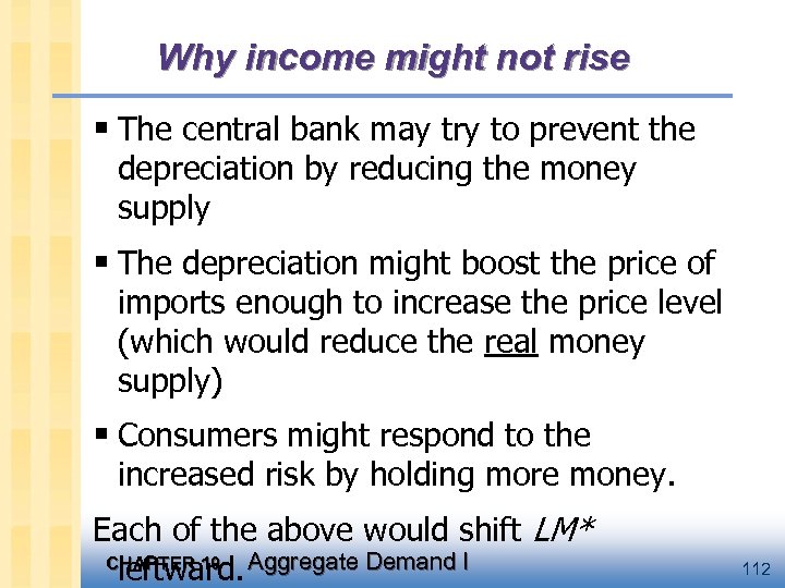 Why income might not rise § The central bank may try to prevent the depreciation by reducing the money supply § The depreciation might boost the price of imports enough to increase the price level (which would reduce the real money supply) § Consumers might respond to the increased risk by holding more money. Each of the above would shift LM* CHAPTER 10 Aggregate Demand I leftward. 112
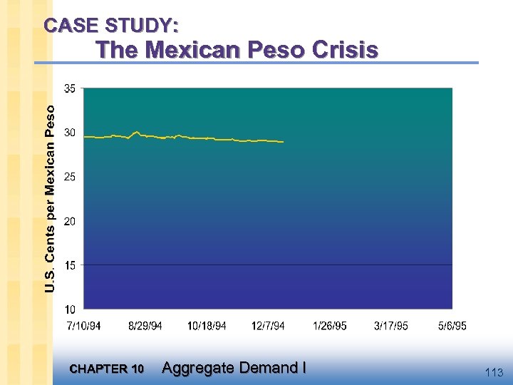 CASE STUDY: The Mexican Peso Crisis CHAPTER 10 Aggregate Demand I 113
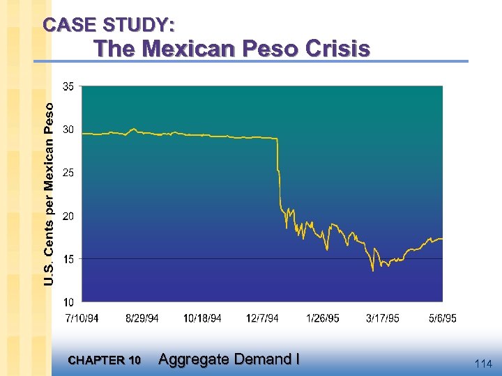 CASE STUDY: The Mexican Peso Crisis CHAPTER 10 Aggregate Demand I 114
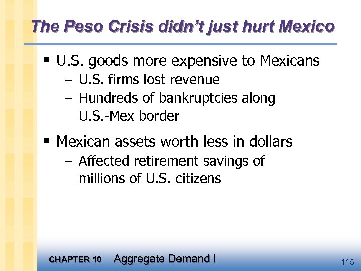 The Peso Crisis didn’t just hurt Mexico § U. S. goods more expensive to Mexicans – U. S. firms lost revenue – Hundreds of bankruptcies along U. S. -Mex border § Mexican assets worth less in dollars – Affected retirement savings of millions of U. S. citizens CHAPTER 10 Aggregate Demand I 115
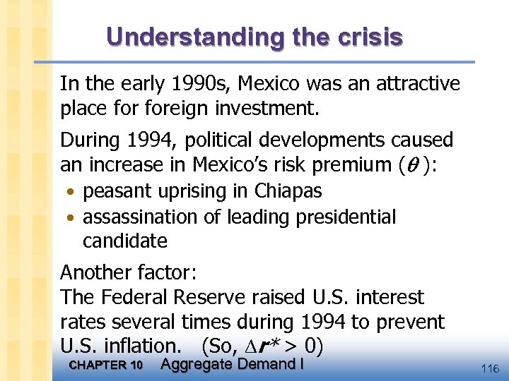 Understanding the crisis In the early 1990 s, Mexico was an attractive place foreign investment. During 1994, political developments caused an increase in Mexico’s risk premium ( ): • peasant uprising in Chiapas • assassination of leading presidential candidate Another factor: The Federal Reserve raised U. S. interest rates several times during 1994 to prevent U. S. inflation. (So, r* > 0) CHAPTER 10 Aggregate Demand I 116
 Understanding the crisis § These events put downward pressure on the peso. § Mexico’s central bank had repeatedly promised foreign investors that it would not allow the peso’s value to fall, so it bought pesos and sold dollars to “prop up” the peso exchange rate. § Doing this requires that Mexico’s central bank have adequate reserves of dollars. Did it? CHAPTER 10 Aggregate Demand I 117
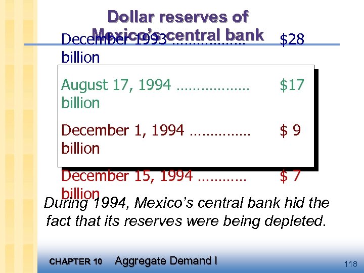 Dollar reserves of Mexico’s ……………… December 1993 central bank $28 billion August 17, 1994 ……………… billion $17 December 1, 1994 …………… billion $9 December 15, 1994 ………… $7 billion During 1994, Mexico’s central bank hid the fact that its reserves were being depleted. CHAPTER 10 Aggregate Demand I 118
 the disaster § Dec. 20: Mexico devalues the peso by 13% (fixes e at 25 cents instead of 29 cents) § Investors are shocked ! ! ! …and realize the central bank must be running out of reserves… § , Investors dump their Mexican assets and pull their capital out of Mexico. § Dec. 22: central bank’s reserves nearly gone. It abandons the fixed rate and lets e float. §CHAPTER 10 Aggregate Demand I 30%. In a week, e falls another 119
 The rescue package § 1995: U. S. & IMF set up $50 b line of credit to provide loan guarantees to Mexico’s govt. § This helped restore confidence in Mexico, reduced the risk premium. § After a hard recession in 1995, Mexico began a strong recovery from the crisis. CHAPTER 10 Aggregate Demand I 120
 Floating vs. Fixed Exchange Rates Argument for floating rates: § allows monetary policy to be used to pursue other goals (stable growth, low inflation) Arguments for fixed rates: § avoids uncertainty and volatility, making international transactions easier § disciplines monetary policy to prevent excessive money growth & hyperinflation CHAPTER 10 Aggregate Demand I 122
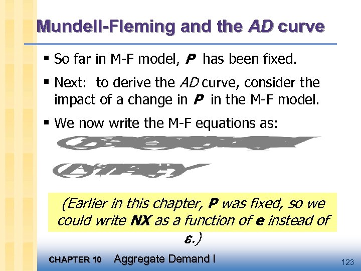 Mundell-Fleming and the AD curve § So far in M-F model, P has been fixed. § Next: to derive the AD curve, consider the impact of a change in P in the M-F model. § We now write the M-F equations as: (Earlier in this chapter, P was fixed, so we could write NX as a function of e instead of . ) CHAPTER 10 Aggregate Demand I 123
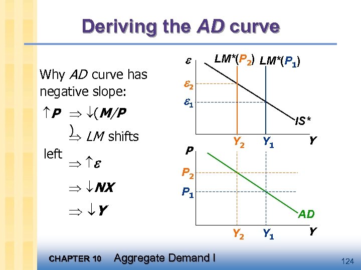 Deriving the AD curve Why AD curve has negative slope: P (M/P ) LM shifts left NX LM*(P 2) LM*(P 1) 2 1 IS* P Y 2 Y 1 P 2 P 1 Y AD Y 2 CHAPTER 10 Y Aggregate Demand I Y 124
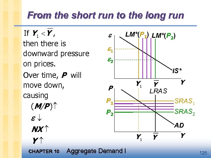 From the short run to the long run there is downward pressure on prices. Over time, P will move down, causing (M/P ) LM*(P 1) LM*(P 2) 1 2 IS* P LRAS P 1 SRAS 1 P 2 SRAS 2 AD NX Y Y CHAPTER 10 Y Aggregate Demand I 125
 Large: between small and closed § Many countries - including the U. S. - are neither closed nor small open economies. § A large open economy is in between the polar cases of closed & small open. § Consider a monetary expansion: • Like in a closed economy, M > 0 r I (though not as much) • Like in a small open economy, M > 0 NX (though not as much) CHAPTER 10 Aggregate Demand I 126
 Chapter summary 1. Mundell-Fleming model § the IS-LM model for a small open economy. § takes P as given § can show policies and shocks affect income and the exchange rate 2. Fiscal policy § affects income under fixed exchange rates, but not under floating exchange rates. CHAPTER 10 Aggregate Demand I 127
 Chapter summary 3. Monetary policy § affects income under floating exchange rates. § Under fixed exchange rates, monetary policy is not available to affect output. 4. Interest rate differentials § exist if investors require a risk premium to hold a country’s assets. § An increase in this risk premium raises domestic interest rates and causes the country’s exchange rate to depreciate. CHAPTER 10 Aggregate Demand I 128
 Chapter summary 5. Fixed vs. floating exchange rates § Under floating rates, monetary policy is available for can purposes other than maintaining exchange rate stability. § Fixed exchange rates reduce some of the uncertainty in international transactions. CHAPTER 10 Aggregate Demand I 129
 CHAPTER 10 Aggregate Demand I 130
 macro CHAPTER TEN Aggregate Demand I macroeconomics fifth edition N. Gregory Mankiw Power. Point® Slides by Ron Cronovich © 2004 Worth Publishers, all rights reserved
 Chapter objectives § difference between short run & long run § introduction to aggregate demand § aggregate supply in the short run & long run § see how model of aggregate supply and demand can be used to analyze short-run and long-run effects of “shocks” CHAPTER 10 Aggregate Demand I 132
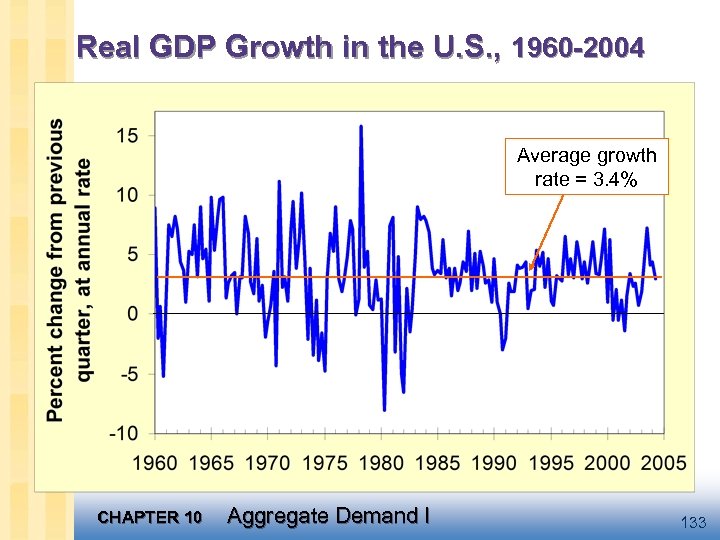 Real GDP Growth in the U. S. , 1960 -2004 Average growth rate = 3. 4% CHAPTER 10 Aggregate Demand I 133
 Time horizons § Long run: Prices are flexible, respond to changes in supply or demand § Short run: many prices are “sticky” at some predetermined level The economy behaves much differently when prices are sticky. CHAPTER 10 Aggregate Demand I 135
 In Classical Macroeconomic Theory, (what we studied in chapters 3 -8) § Output is determined by the supply side: – supplies of capital, labor – technology § Changes in demand for goods & services (C, I, G ) only affect prices, not quantities. § Complete price flexibility is a crucial assumption, so classical theory applies in the long run. CHAPTER 10 Aggregate Demand I 136
 When prices are sticky …output and employment also depend on demand for goods & services, which is affected by § fiscal policy (G and T ) § monetary policy (M ) § other factors, like exogenous changes in C or I. CHAPTER 10 Aggregate Demand I 137
 The model of aggregate demand supply § the paradigm that most mainstream economists & policymakers use to think about economic fluctuations and policies to stabilize the economy § shows how the price level and aggregate output are determined § shows how the economy’s behavior is different in the short run and long run CHAPTER 10 Aggregate Demand I 138
 Aggregate demand § The aggregate demand curve shows the relationship between the price level and the quantity of output demanded. § For this chapter’s intro to the AD/AS model, we use a simple theory of aggregate demand based on the Quantity Theory of Money. § Chapters 10 -12 develop theory of aggregate demand in more detail. CHAPTER 10 Aggregate Demand I 139
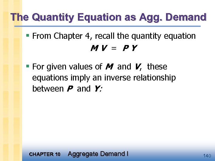 The Quantity Equation as Agg. Demand § From Chapter 4, recall the quantity equation MV = PY § For given values of M and V, these equations imply an inverse relationship between P and Y: CHAPTER 10 Aggregate Demand I 140
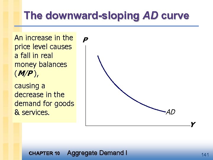 The downward-sloping AD curve An increase in the price level causes a fall in real money balances (M/P ), P causing a decrease in the demand for goods & services. AD Y CHAPTER 10 Aggregate Demand I 141
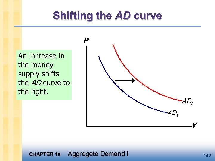 Shifting the AD curve P An increase in the money supply shifts the AD curve to the right. AD 2 AD 1 Y CHAPTER 10 Aggregate Demand I 142
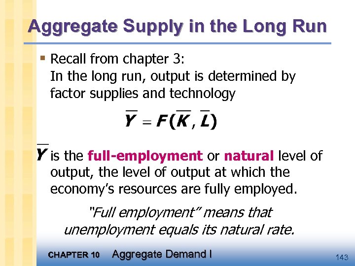 Aggregate Supply in the Long Run § Recall from chapter 3: In the long run, output is determined by factor supplies and technology is the full-employment or natural level of output, the level of output at which the economy’s resources are fully employed. “Full employment” means that unemployment equals its natural rate. CHAPTER 10 Aggregate Demand I 143
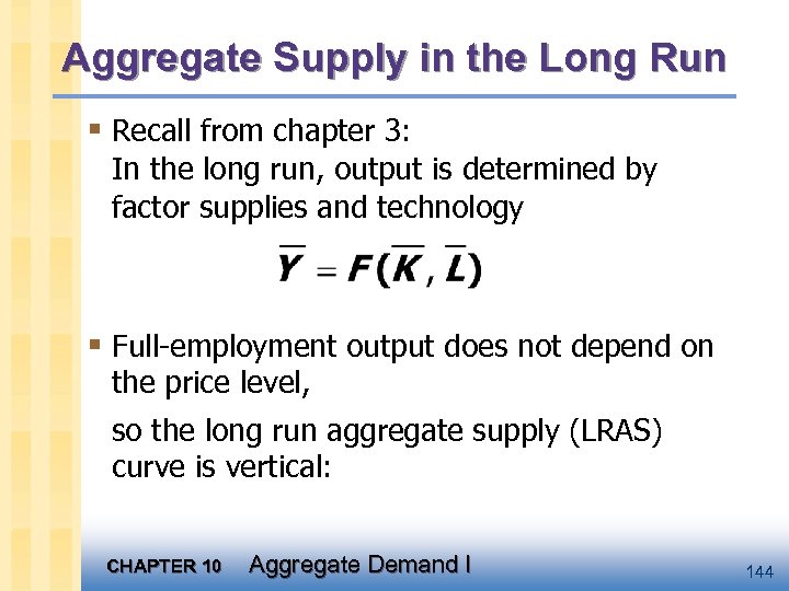 Aggregate Supply in the Long Run § Recall from chapter 3: In the long run, output is determined by factor supplies and technology § Full-employment output does not depend on the price level, so the long run aggregate supply (LRAS) curve is vertical: CHAPTER 10 Aggregate Demand I 144
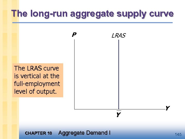 The long-run aggregate supply curve P LRAS The LRAS curve is vertical at the full-employment level of output. Y CHAPTER 10 Aggregate Demand I 145
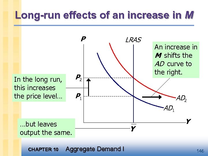 Long-run effects of an increase in M P P 2 In the long run, this increases the price level… LRAS An increase in M shifts the AD curve to the right. P 1 AD 2 AD 1 …but leaves output the same. CHAPTER 10 Aggregate Demand I Y 146
 Aggregate Supply in the Short Run § In the real world, many prices are sticky in the short run. § For now (and throughout Chapters 9 -12), we assume that all prices are stuck at a predetermined level in the short run… § …and that firms are willing to sell as much at that price level as their customers are willing to buy. § Therefore, the short-run aggregate supply (SRAS) curve is horizontal: CHAPTER 10 Aggregate Demand I 147
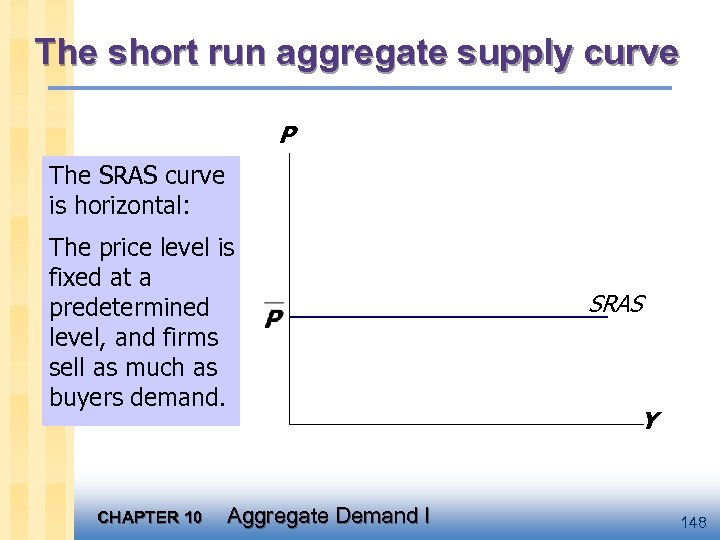 The short run aggregate supply curve P The SRAS curve is horizontal: The price level is fixed at a predetermined level, and firms sell as much as buyers demand. CHAPTER 10 Aggregate Demand I SRAS Y 148
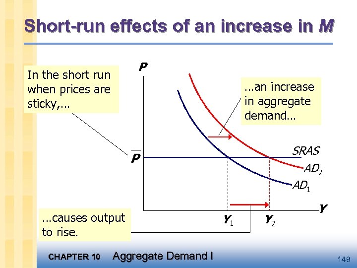 Short-run effects of an increase in M P In the short run when prices are sticky, … …an increase in aggregate demand… SRAS AD 2 AD 1 …causes output to rise. CHAPTER 10 Aggregate Demand I Y 1 Y 2 Y 149
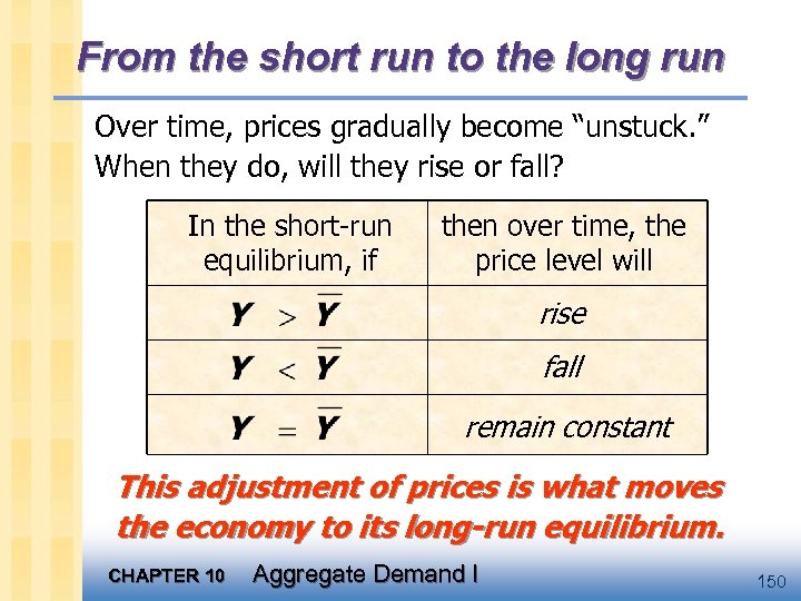 From the short run to the long run Over time, prices gradually become “unstuck. ” When they do, will they rise or fall? In the short-run equilibrium, if then over time, the price level will rise fall remain constant This adjustment of prices is what moves the economy to its long-run equilibrium. CHAPTER 10 Aggregate Demand I 150
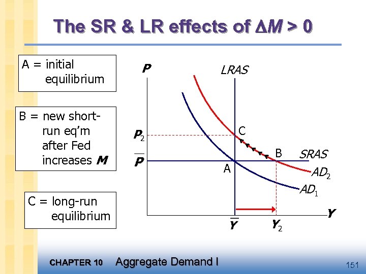 The SR & LR effects of M > 0 A = initial equilibrium B = new shortrun eq’m after Fed increases M P C P 2 B A C = long-run equilibrium CHAPTER 10 LRAS Y 2 Aggregate Demand I SRAS AD 2 AD 1 Y 151
 How shocking!!! § shocks: exogenous changes in aggregate supply or demand § Shocks temporarily push the economy away from full-employment. § An example of a demand shock: exogenous decrease in velocity § If the money supply is held constant, then a decrease in V means people will be using their money in fewer transactions, causing a decrease in demand for goods and services: CHAPTER 10 Aggregate Demand I 152
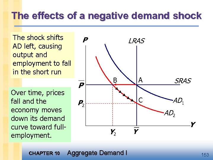 The effects of a negative demand shock The shock shifts AD left, causing output and employment to fall in the short run P LRAS Over time, prices fall and the economy moves down its demand curve toward fullemployment. CHAPTER 10 P 2 A SRAS C B AD 1 AD 2 Y 2 Aggregate Demand I Y 153
 Supply shocks A supply shock alters production costs, affects the prices that firms charge. (also called price shocks) Examples of adverse supply shocks: § Bad weather reduces crop yields, pushing up food prices. § Workers unionize, negotiate wage increases. § New environmental regulations require firms to reduce emissions. Firms charge higher prices to help cover the costs of compliance. (Favorable supply shocks lower costs and prices. ) CHAPTER 10 Aggregate Demand I 154
 CASE STUDY: The 1970 s oil shocks § Early 1970 s: OPEC coordinates a reduction in the supply of oil. § Oil prices rose 11% in 1973 68% in 1974 16% in 1975 § Such sharp oil price increases are supply shocks because they significantly impact production costs and prices. CHAPTER 10 Aggregate Demand I 155
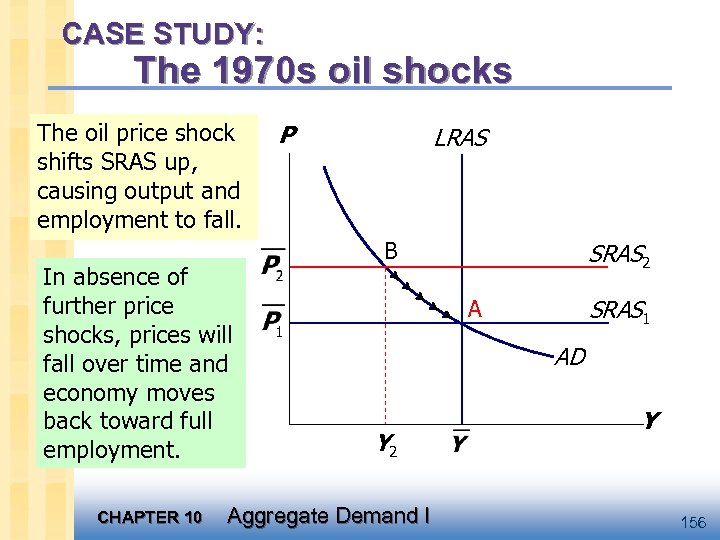 CASE STUDY: The 1970 s oil shocks The oil price shock shifts SRAS up, causing output and employment to fall. In absence of further price shocks, prices will fall over time and economy moves back toward full employment. CHAPTER 10 P LRAS B SRAS 2 SRAS 1 A AD Y 2 Aggregate Demand I Y 156
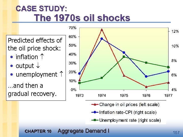 CASE STUDY: The 1970 s oil shocks Predicted effects of the oil price shock: • inflation • output • unemployment …and then a gradual recovery. CHAPTER 10 Aggregate Demand I 157
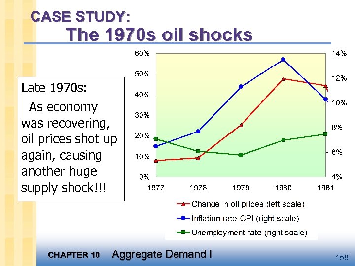 CASE STUDY: The 1970 s oil shocks Late 1970 s: As economy was recovering, oil prices shot up again, causing another huge supply shock!!! CHAPTER 10 Aggregate Demand I 158
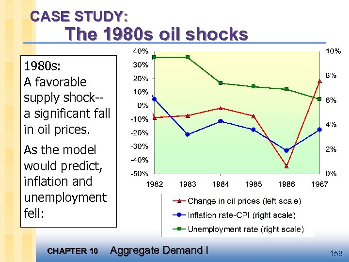 CASE STUDY: The 1980 s oil shocks 1980 s: A favorable supply shock-a significant fall in oil prices. As the model would predict, inflation and unemployment fell: CHAPTER 10 Aggregate Demand I 159
 Stabilization policy § def: policy actions aimed at reducing the severity of short-run economic fluctuations. § Example: Using monetary policy to combat the effects of adverse supply shocks: CHAPTER 10 Aggregate Demand I 160
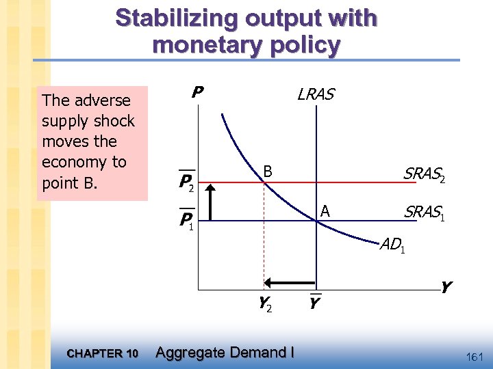 Stabilizing output with monetary policy The adverse supply shock moves the economy to point B. P LRAS B SRAS 2 A SRAS 1 AD 1 Y 2 CHAPTER 10 Aggregate Demand I Y 161
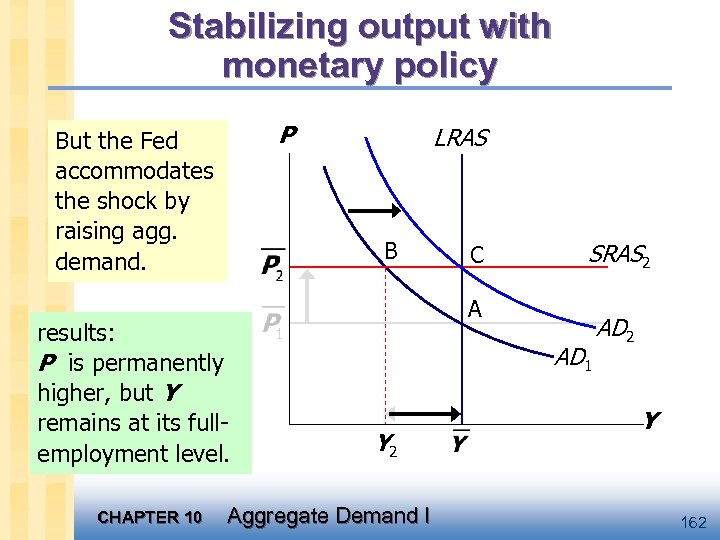 Stabilizing output with monetary policy P But the Fed accommodates the shock by raising agg. demand. B results: P is permanently higher, but Y remains at its fullemployment level. CHAPTER 10 LRAS C SRAS 2 A AD 1 Y 2 Aggregate Demand I AD 2 Y 162
 Chapter summary 1. Long run: prices are flexible, output and employment are always at their natural rates, and the classical theory applies. Short run: prices are sticky, shocks can push output and employment away from their natural rates. 2. Aggregate demand supply: a framework to analyze economic fluctuations CHAPTER 10 Aggregate Demand I 163
 Chapter summary 3. The aggregate demand curve slopes downward. 4. The long-run aggregate supply curve is vertical, because output depends on technology and factor supplies, but not prices. 5. The short-run aggregate supply curve is horizontal, because prices are sticky at predetermined levels. CHAPTER 10 Aggregate Demand I 164
 Chapter summary 6. Shocks to aggregate demand supply cause fluctuations in GDP and employment in the short run. 7. The Fed can attempt to stabilize the economy with monetary policy. CHAPTER 10 Aggregate Demand I 165
 CHAPTER 10 Aggregate Demand I 166


