Machine Learning Neural Networks Tomorrow no lesson will

Machine Learning Neural Networks Tomorrow no lesson! (will recover on Wednesday 11, WEKA !!) 1

Neural Networks • Analogy to biological neural systems, the most robust learning systems we know. • Attempt to understand natural biological systems through computational modeling. • Massive parallelism allows for computational efficiency. • Help understand “distributed” nature of neural representations (rather than “localist” representation) that allow robustness and graceful degradation. • Intelligent behavior as an “emergent” property of large number of simple units rather than from explicitly encoded symbolic rules and algorithms. 2

Neural Speed Constraints • Neurons have a “switching time” on the order of a few milliseconds, compared to nanoseconds for current computing hardware. • However, neural systems can perform complex cognitive tasks (vision, speech understanding) in tenths of a second. • Only time for performing 100 serial steps in this time frame, compared to orders of magnitude more for current computers. • Must be exploiting “massive parallelism. ” • Human brain has about 1011 neurons with an average of 104 connections each. 3

Neural Network Learning • Learning approach based on modeling adaptation in biological neural systems. • Perceptron: Initial algorithm for learning simple neural networks (single layer) developed in the 1950’s. • Backpropagation: More complex algorithm for learning multi-layer neural networks developed in the 1980’s. 4

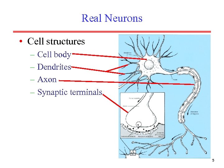Real Neurons • Cell structures – Cell body – Dendrites – Axon – Synaptic terminals 5

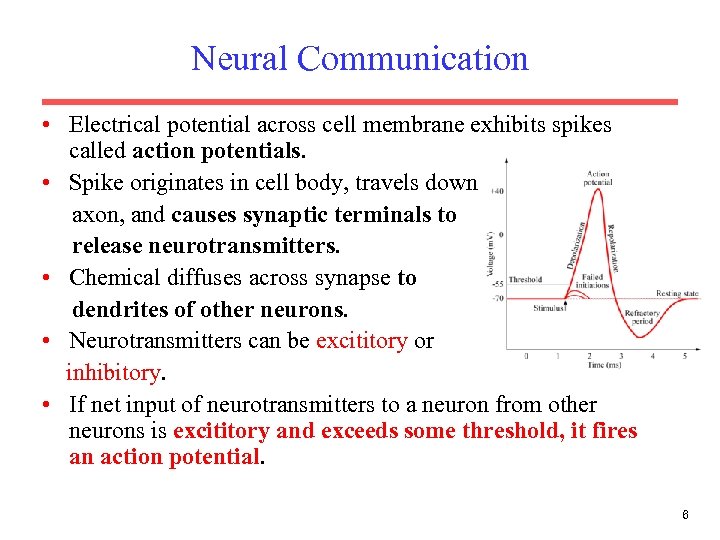Neural Communication • Electrical potential across cell membrane exhibits spikes called action potentials. • Spike originates in cell body, travels down axon, and causes synaptic terminals to release neurotransmitters. • Chemical diffuses across synapse to dendrites of other neurons. • Neurotransmitters can be excititory or inhibitory. • If net input of neurotransmitters to a neuron from other neurons is excititory and exceeds some threshold, it fires an action potential. 6

Real Neural Learning • Synapses change size and strength with experience. • Hebbian learning: When two connected neurons are firing at the same time, the strength of the synapse between them increases. • “Neurons that fire together, wire together. ” 7

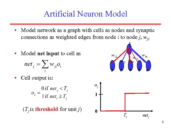Artificial Neuron Model • Model network as a graph with cells as nodes and synaptic connections as weighted edges from node i to node j, wji 1 • Model net input to cell as w 12 2 w 15 w 13 w 14 3 4 5 w 16 6 • Cell output is: oj 1 (Tj is threshold for unit j) 0 Tj netj 8

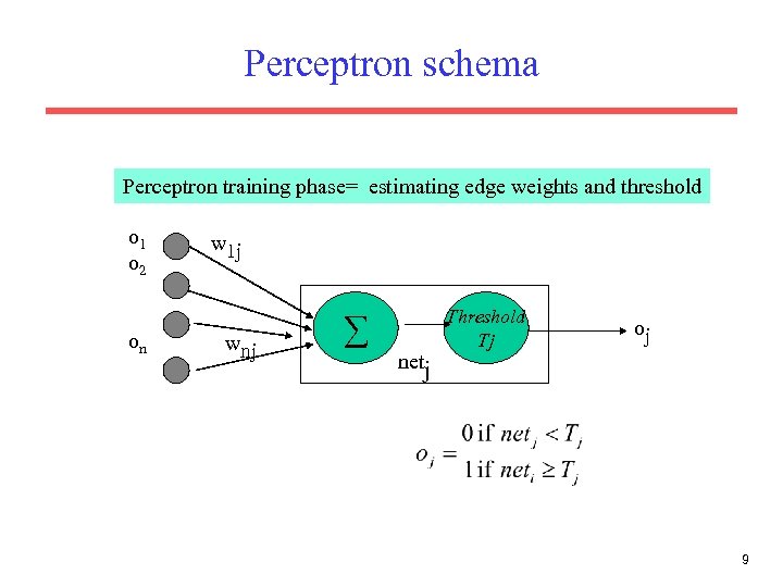Perceptron schema Perceptron training phase= estimating edge weights and threshold o 1 o 2 on w 1 j wnj ∑ netj Threshold Tj oj 9

Perceptron Training • Assume supervised training examples giving the desired output for a unit given a set of known input activations. • Learn synaptic weights so that unit produces the correct output for each example. • Perceptron uses iterative update algorithm to learn a correct set of weights. 10

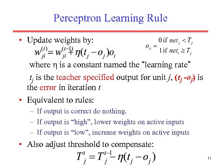Perceptron Learning Rule • Update weights by: where η is a constant named the “learning rate” tj is the teacher specified output for unit j, (tj -oj) is the error in iteration t • Equivalent to rules: – If output is correct do nothing. – If output is “high”, lower weights on active inputs – If output is “low”, increase weights on active inputs • Also adjust threshold to compensate: 11

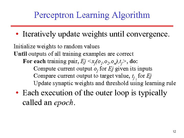Perceptron Learning Algorithm • Iteratively update weights until convergence. Initialize weights to random values Until outputs of all training examples are correct For each training pair, Ej , do: Compute current output oj for Ej given its inputs Compare current output to target value, tj , for Ej Update synaptic weights and threshold using learning rule • Each execution of the outer loop is typically called an epoch. 12

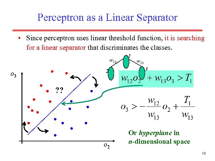Perceptron as a Linear Separator • Since perceptron uses linear threshold function, it is searching for a linear separator that discriminates the classes. w 12 2 o 3 1 w 13 3 ? ? o 2 Or hyperplane in n-dimensional space 13

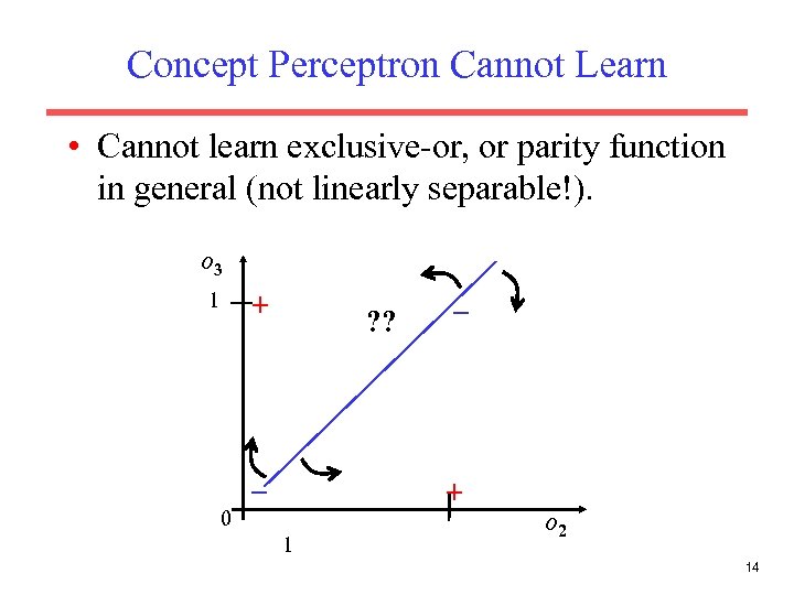Concept Perceptron Cannot Learn • Cannot learn exclusive-or, or parity function in general (not linearly separable!). o 3 + 1 0 ? ? – – + 1 o 2 14

Perceptron Limits • System obviously cannot learn concepts it cannot represent. • Minksy and Papert (1969) wrote a book analyzing the perceptron and demonstrating many functions it could not learn. • These results discouraged further research on neural nets; and symbolic AI became the dominate paradigm. 15

Perceptron Convergence and Cycling Theorems • Perceptron convergence theorem: If the data is linearly separable and therefore a set of weights exist that are consistent with the data, then the Perceptron algorithm will eventually converge to a consistent set of weights. • Perceptron cycling theorem: If the data is not linearly separable, the Perceptron algorithm will eventually repeat a set of weights and threshold at the end of some epoch and therefore enter an infinite loop. – By checking for repeated weights+threshold, one can guarantee termination with either a positive or negative result. 16

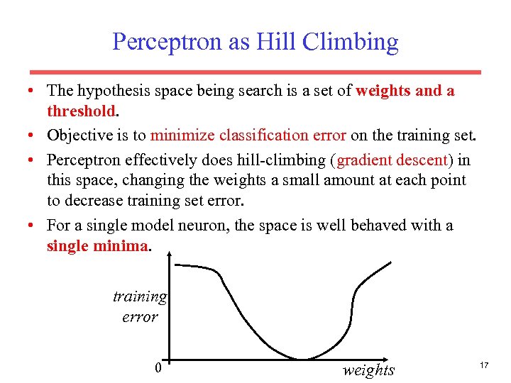Perceptron as Hill Climbing • The hypothesis space being search is a set of weights and a threshold. • Objective is to minimize classification error on the training set. • Perceptron effectively does hill-climbing (gradient descent) in this space, changing the weights a small amount at each point to decrease training set error. • For a single model neuron, the space is well behaved with a single minima. training error 0 weights 17

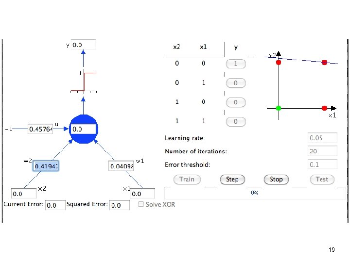
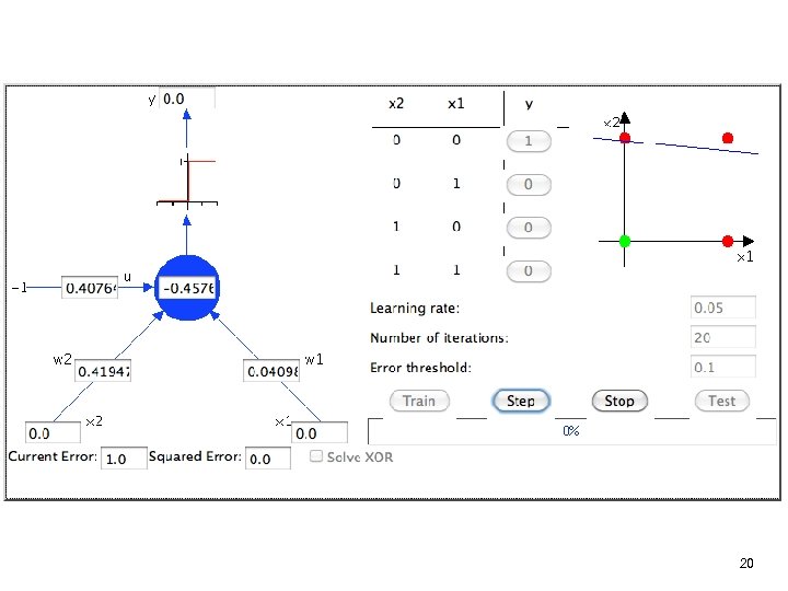
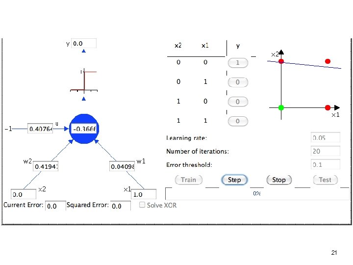
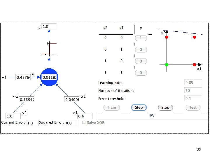
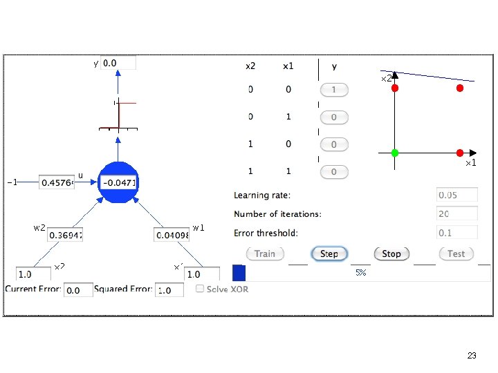
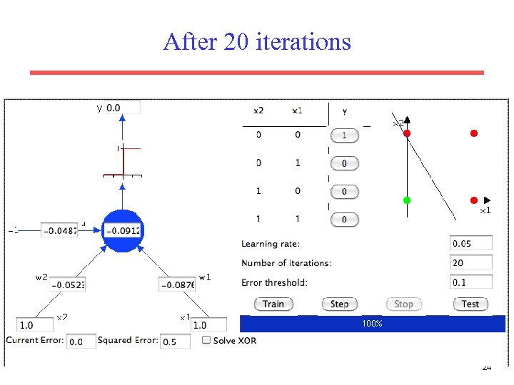
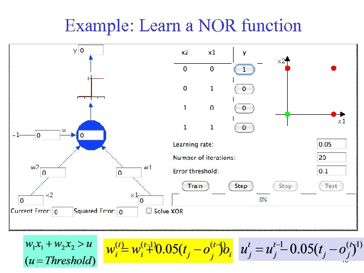Example: Learn a NOR function 18

19

20

21

22

23

After 20 iterations 24

Perceptron Performance • In practice, converges fairly quickly for linearly separable data. • Can effectively use even incompletely converged results when only a few outliers are misclassified. • Experimentally, Perceptron does quite well on many benchmark data sets. 25

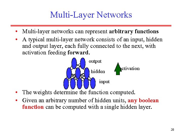Multi-Layer Networks • Multi-layer networks can represent arbitrary functions • A typical multi-layer network consists of an input, hidden and output layer, each fully connected to the next, with activation feeding forward. output hidden activation input • The weights determine the function computed. • Given an arbitrary number of hidden units, any boolean function can be computed with a single hidden layer. 26

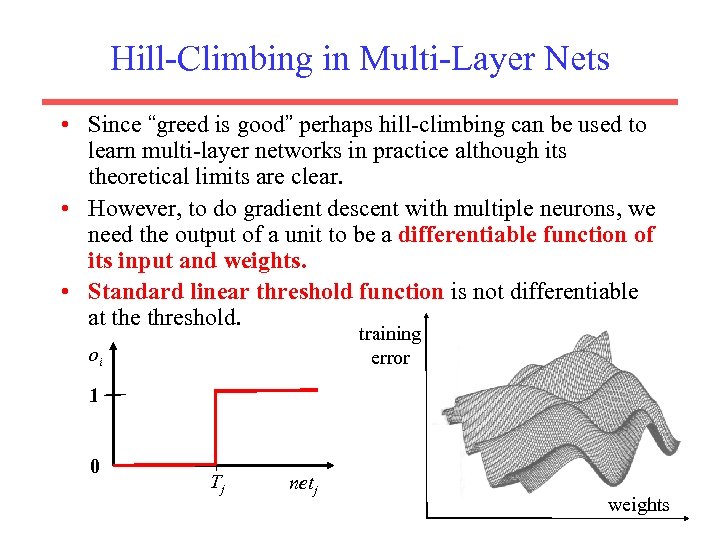Hill-Climbing in Multi-Layer Nets • Since “greed is good” perhaps hill-climbing can be used to learn multi-layer networks in practice although its theoretical limits are clear. • However, to do gradient descent with multiple neurons, we need the output of a unit to be a differentiable function of its input and weights. • Standard linear threshold function is not differentiable at the threshold. training error oi 1 0 Tj netj weights 27

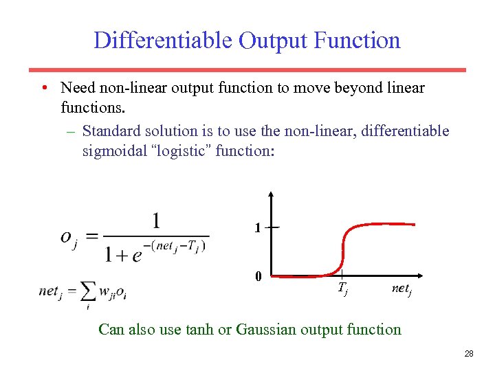Differentiable Output Function • Need non-linear output function to move beyond linear functions. – Standard solution is to use the non-linear, differentiable sigmoidal “logistic” function: 1 0 Tj netj Can also use tanh or Gaussian output function 28

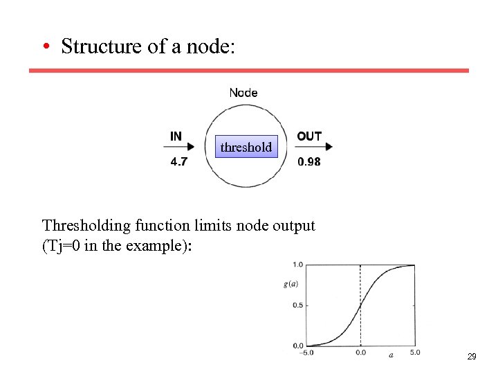• Structure of a node: threshold Thresholding function limits node output (Tj=0 in the example): 29

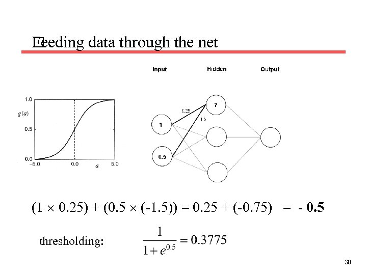Feeding data through the net (1 0. 25) + (0. 5 (-1. 5)) = 0. 25 + (-0. 75) = - 0. 5 thresholding: 30

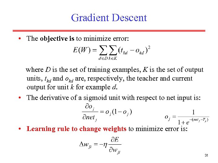Gradient Descent • The objective is to minimize error: where D is the set of training examples, K is the set of output units, tkd and okd are, respectively, the teacher and current output for unit k for example d. • The derivative of a sigmoid unit with respect to net input is: • Learning rule to change weights to minimize error is: 31

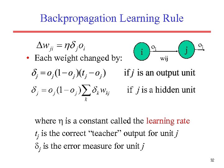Backpropagation Learning Rule • Each weight changed by: i oi j oj wij where η is a constant called the learning rate tj is the correct “teacher” output for unit j δj is the error measure for unit j 32

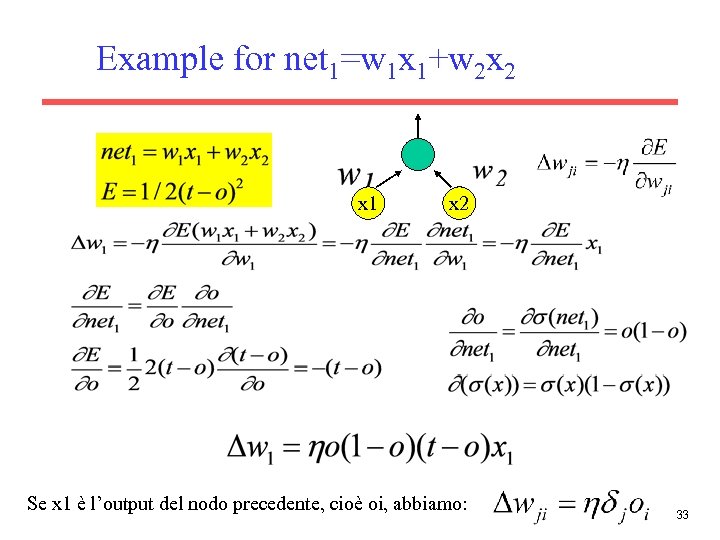Example for net 1=w 1 x 1+w 2 x 2 x 1 x 2 Se x 1 è l’output del nodo precedente, cioè oi, abbiamo: 33

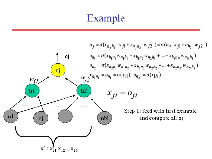Example oj nj wj 1 wj 2 h 1 h 2 ……. n 1 …. . . nj x 1: x 11 x 12…x 1 N …. . n. N Step 1: feed with first example and compute all oj

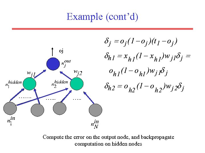Example (cont’d) oj wj 2 wj 1 ……. …. . Compute the error on the output node, and backpropagate computation on hidden nodes

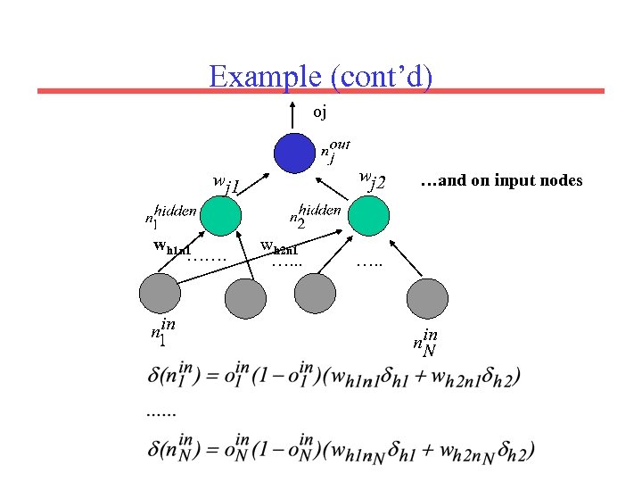Example (cont’d) oj wj 2 wj 1 wh 1 n 1 ……. wh 2 n 1 …. . . …and on input nodes

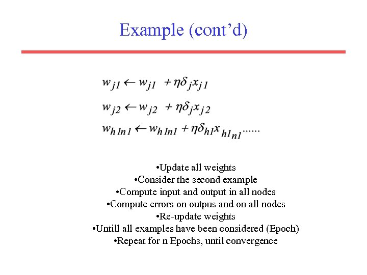Example (cont’d) • Update all weights • Consider the second example • Compute input and output in all nodes • Compute errors on outpus and on all nodes • Re-update weights • Untill all examples have been considered (Epoch) • Repeat for n Epochs, until convergence

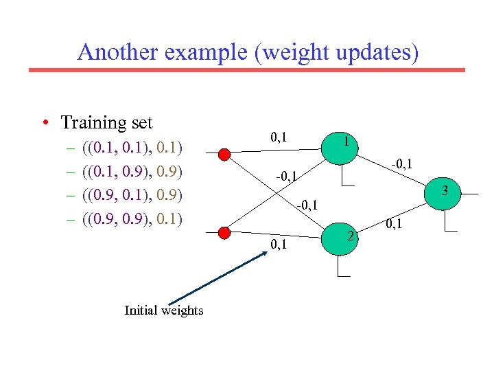Another example (weight updates) • Training set – – ((0. 1, 0. 1) ((0. 1, 0. 9) ((0. 9, 0. 1), 0. 9) ((0. 9, 0. 9), 0. 1) 0, 1 -0, 1 3 -0, 1 Initial weights 1 2 0, 1

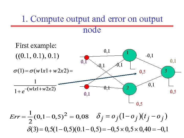1. Compute output and error on output node First example: ((0. 1, 0. 1) 0, 1 -0, 1 3 0, 5 0, 1 2 0, 5 0, 1 0, 5

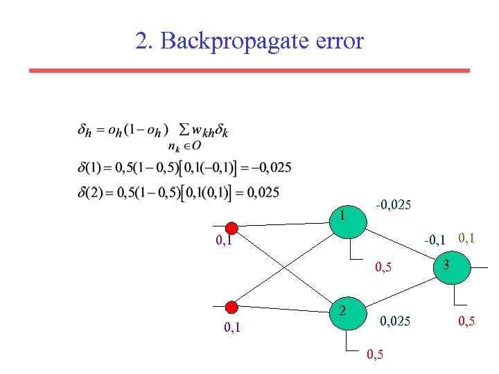2. Backpropagate error 1 -0, 025 -0, 1 0, 5 2 0, 1 0, 025 0, 5 3 0, 5

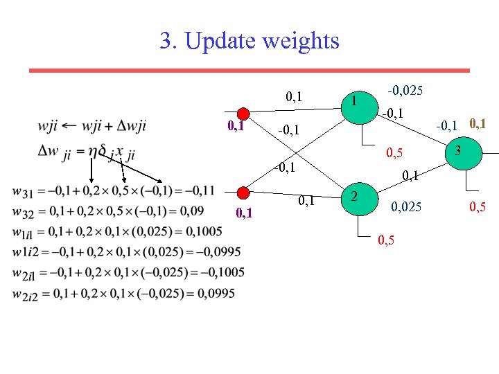3. Update weights 0, 1 1 -0, 1 0, 5 -0, 1 -0, 025 -0, 1 3 0, 1 2 0, 025 0, 5

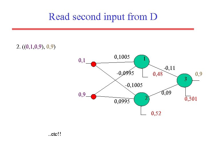Read second input from D 2. ((0, 1, 0, 9) 0, 1005 1 -0, 0995 0, 48 -0, 11 -0, 1005 0, 9 0, 0995 0, 09 2 0, 52 . . etc!! 3 0, 9 0, 501

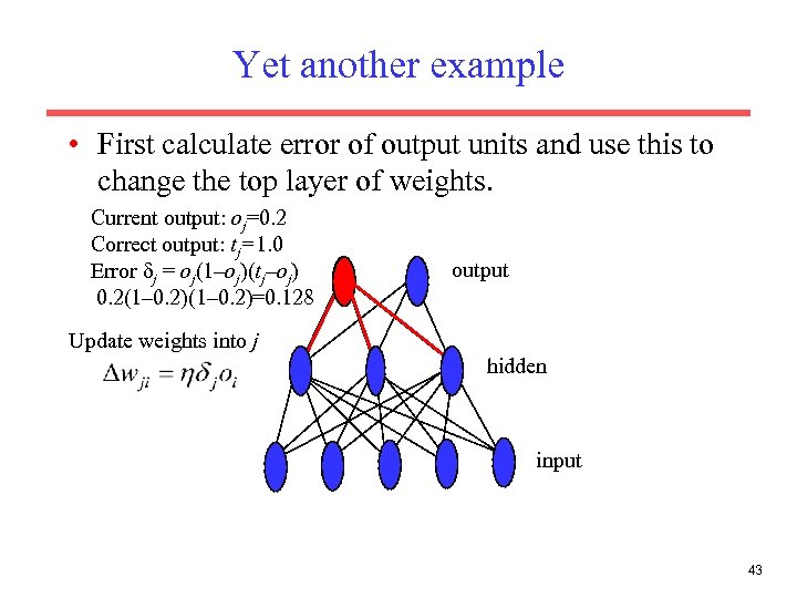Yet another example • First calculate error of output units and use this to change the top layer of weights. Current output: oj=0. 2 Correct output: tj=1. 0 Error δj = oj(1–oj)(tj–oj) 0. 2(1– 0. 2)=0. 128 output Update weights into j hidden input 43

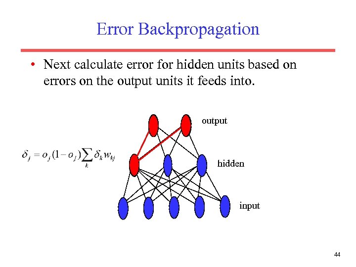Error Backpropagation • Next calculate error for hidden units based on errors on the output units it feeds into. output hidden input 44

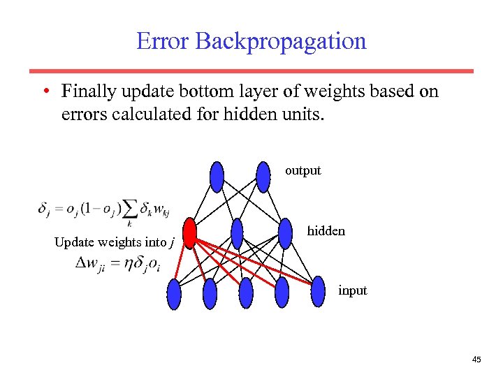Error Backpropagation • Finally update bottom layer of weights based on errors calculated for hidden units. output Update weights into j hidden input 45

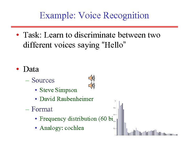Example: Voice Recognition • Task: Learn to discriminate between two different voices saying “Hello” • Data – Sources • Steve Simpson • David Raubenheimer – Format • Frequency distribution (60 bins) • Analogy: cochlea

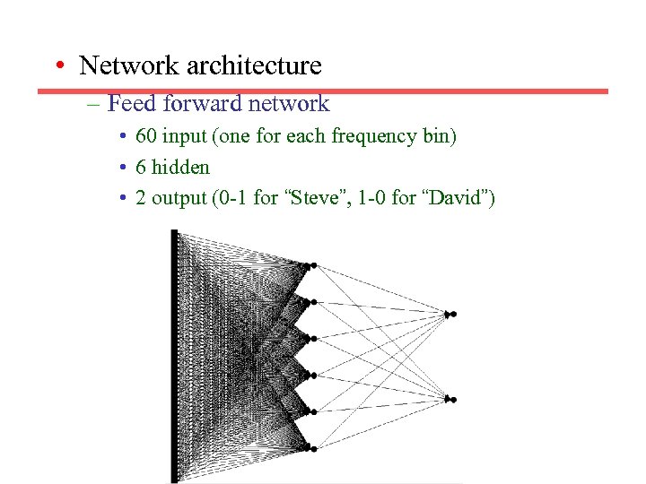• Network architecture – Feed forward network • 60 input (one for each frequency bin) • 6 hidden • 2 output (0 -1 for “Steve”, 1 -0 for “David”)

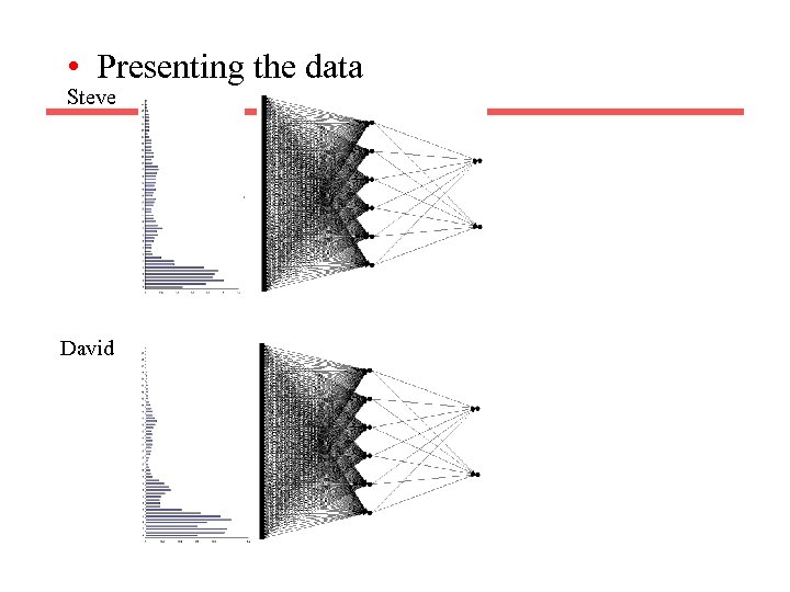• Presenting the data Steve David

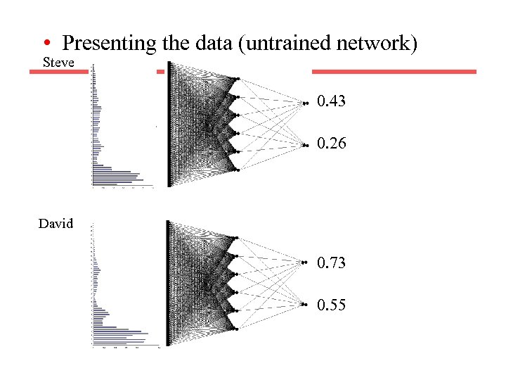• Presenting the data (untrained network) Steve 0. 43 0. 26 David 0. 73 0. 55

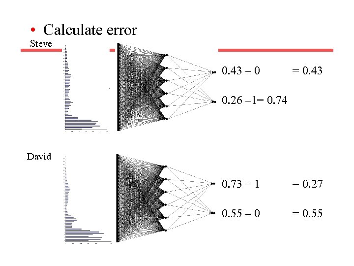• Calculate error Steve 0. 43 – 0 = 0. 43 0. 26 – 1= 0. 74 David 0. 73 – 1 = 0. 27 0. 55 – 0 = 0. 55

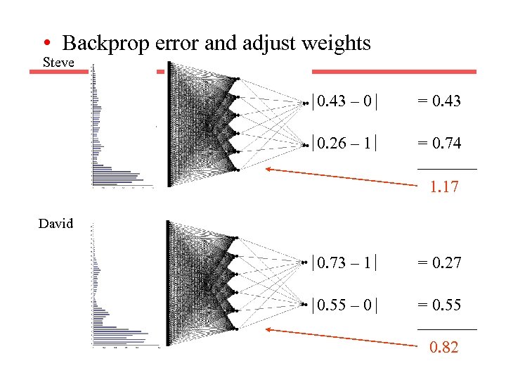• Backprop error and adjust weights Steve 0. 43 – 0 = 0. 43 0. 26 – 1 = 0. 74 1. 17 David 0. 73 – 1 = 0. 27 0. 55 – 0 = 0. 55 0. 82

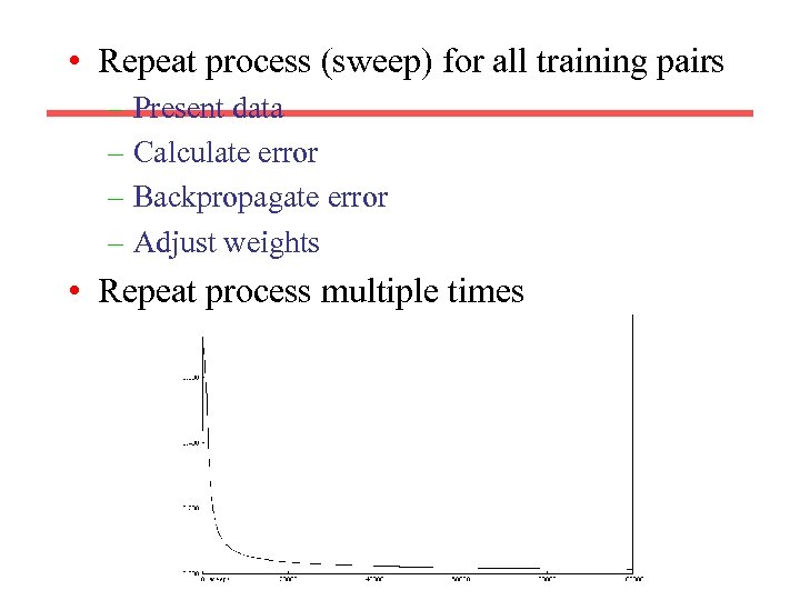• Repeat process (sweep) for all training pairs – Present data – Calculate error – Backpropagate error – Adjust weights • Repeat process multiple times

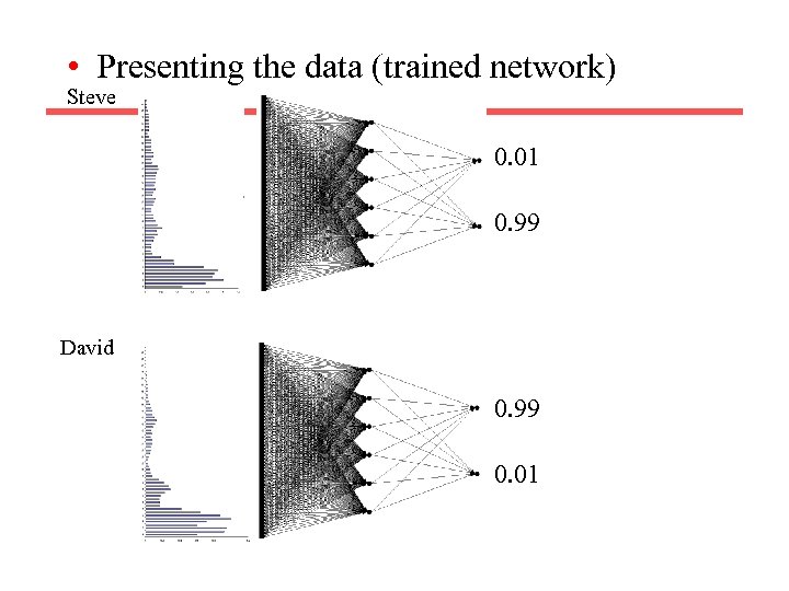• Presenting the data (trained network) Steve 0. 01 0. 99 David 0. 99 0. 01

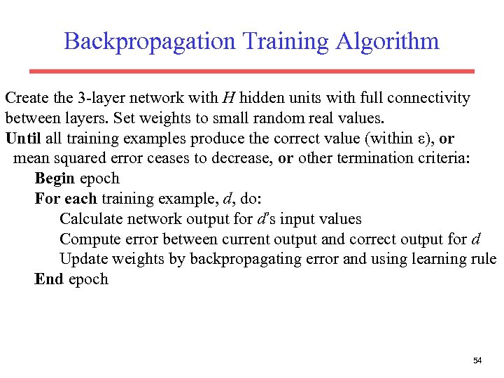Backpropagation Training Algorithm Create the 3 -layer network with H hidden units with full connectivity between layers. Set weights to small random real values. Until all training examples produce the correct value (within ε), or mean squared error ceases to decrease, or other termination criteria: Begin epoch For each training example, d, do: Calculate network output for d’s input values Compute error between current output and correct output for d Update weights by backpropagating error and using learning rule End epoch 54

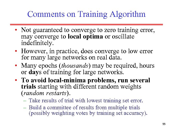Comments on Training Algorithm • Not guaranteed to converge to zero training error, may converge to local optima or oscillate indefinitely. • However, in practice, does converge to low error for many large networks on real data. • Many epochs (thousands) may be required, hours or days of training for large networks. • To avoid local-minima problems, run several trials starting with different random weights (random restarts). – Take results of trial with lowest training set error. – Build a committee of results from multiple trials (possibly weighting votes by training set accuracy). 55

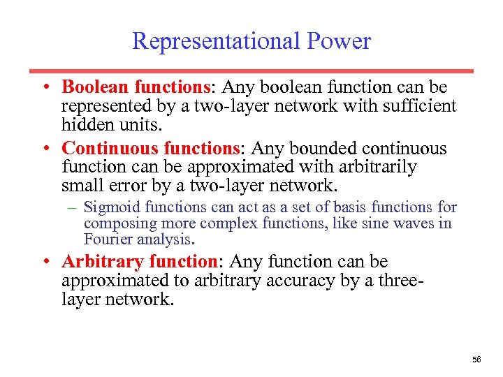Representational Power • Boolean functions: Any boolean function can be represented by a two-layer network with sufficient hidden units. • Continuous functions: Any bounded continuous function can be approximated with arbitrarily small error by a two-layer network. – Sigmoid functions can act as a set of basis functions for composing more complex functions, like sine waves in Fourier analysis. • Arbitrary function: Any function can be approximated to arbitrary accuracy by a threelayer network. 56

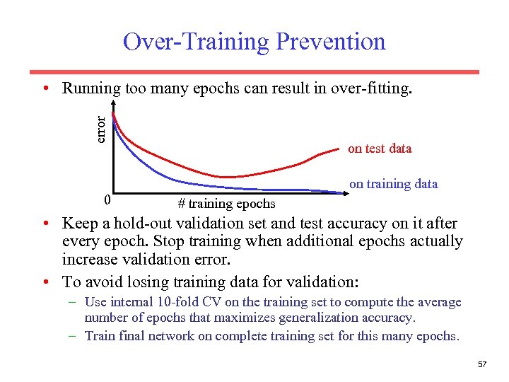Over-Training Prevention error • Running too many epochs can result in over-fitting. on test data on training data 0 # training epochs • Keep a hold-out validation set and test accuracy on it after every epoch. Stop training when additional epochs actually increase validation error. • To avoid losing training data for validation: – Use internal 10 -fold CV on the training set to compute the average number of epochs that maximizes generalization accuracy. – Train final network on complete training set for this many epochs. 57

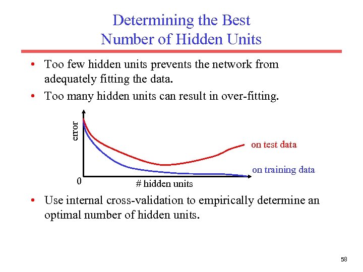Determining the Best Number of Hidden Units error • Too few hidden units prevents the network from adequately fitting the data. • Too many hidden units can result in over-fitting. on test data on training data 0 # hidden units • Use internal cross-validation to empirically determine an optimal number of hidden units. 58

Successful Applications • Text to Speech (Net. Talk) • Fraud detection • Financial Applications – HNC (eventually bought by Fair Isaac) • Chemical Plant Control – Pavillion Technologies • Automated Vehicles • Game Playing – Neurogammon • Handwriting recognition 59

Issues in Neural Nets • More efficient training methods: – Quickprop – Conjugate gradient (exploits 2 nd derivative) • Learning the proper network architecture: – Grow network until able to fit data • Cascade Correlation • Upstart – Shrink large network until unable to fit data • Optimal Brain Damage • Recurrent networks that use feedback and can learn finite state machines with “backpropagation through time. ” 60

Issues in Neural Nets (cont. ) • More biologically plausible learning algorithms based on Hebbian learning. • Unsupervised Learning – Self-Organizing Feature Maps (SOMs) • Reinforcement Learning – Frequently used as function approximators for learning value functions. • Neuroevolution 61