Machine Learning in Natural Language Semi-Supervised Learning and

Machine Learning in Natural Language Semi-Supervised Learning and the EM Algorithm 1

Semi-Supervised Learning n Consider the problem of Prepositional Phrase Attachment. n n Buy car with money ; buy car with steering wheel There are several ways to generate features. Given the limited representation, we can assume that all possible conjunctions of the up to 4 attributes are used. (15 features in each example). Assume we will use naïve Bayes for learning to decide between [n, v] Examples are: (x 1, x 2, …xn, [n, v]) 2

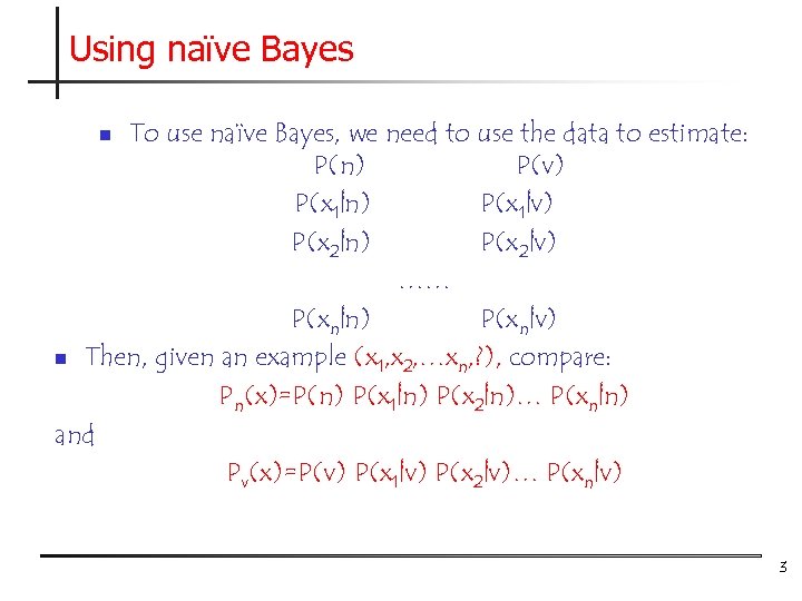Using naïve Bayes To use naïve Bayes, we need to use the data to estimate: P(n) P(v) P(x 1|n) P(x 1|v) P(x 2|n) P(x 2|v) …… P(xn|n) P(xn|v) n Then, given an example (x 1, x 2, …xn, ? ), compare: Pn(x)=P(n) P(x 1|n) P(x 2|n)… P(xn|n) and Pv(x)=P(v) P(x 1|v) P(x 2|v)… P(xn|v) n 3

Using naïve Bayes After seeing 10 examples, we have: n P(n) =0. 5; P(v)=0. 5 P(x 1|n)=0. 75; P(x 2|n) =0. 5; P(x 3|n) =0. 5; P(x 4|n) =0. 5 P(x 1|v)=0. 25; P(x 2|v) =0. 25; P(x 3|v) =0. 75; P(x 4|v) =0. 5 n Then, given an example (1000), we have: Pn(x)=0. 5 0. 75 0. 5 = 3/64 Pv(x)=0. 5 0. 25 0. 75 0. 25 0. 5=3/256 Now, assume that in addition to the 10 labeled examples, we also have 100 unlabeled examples. n 4

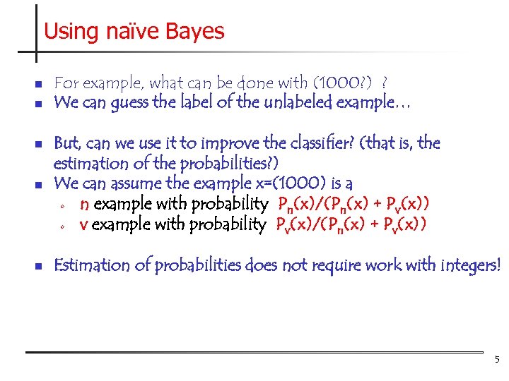Using naïve Bayes n n For example, what can be done with (1000? ) ? We can guess the label of the unlabeled example… n But, can we use it to improve the classifier? (that is, the estimation of the probabilities? ) We can assume the example x=(1000) is a • n example with probability Pn(x)/(Pn(x) + Pv(x)) • v example with probability Pv(x)/(Pn(x) + Pv(x)) n Estimation of probabilities does not require work with integers! n 5

Using Unlabeled Data The discussion suggests several algorithms: 1. 2. Use a threshold. Chose examples labeled with high confidence. Labeled them [n, v]. Retrain. Use fractional examples. Label the examples with fractional labels [p of n, (1 -p) of v]. Retrain. 6

Comments on Unlabeled Data n n n Both algorithms suggested can be used iteratively. Both algorithms can be used with other classifiers, not only naïve Bayes. The only requirement – a robust confidence measure in the classification. E. g. : Brill, ACL’ 01: uses all three algorithms in SNo. W for studies of these sort. 7

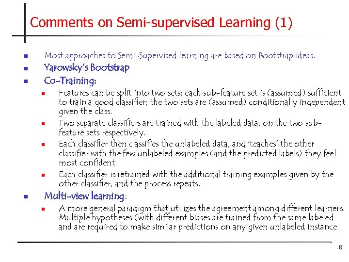Comments on Semi-supervised Learning (1) n n n Most approaches to Semi-Supervised learning are based on Bootstrap ideas. Yarowsky’s Bootstrap Co-Training: n n n Features can be split into two sets; each sub-feature set is (assumed) sufficient to train a good classifier; the two sets are (assumed) conditionally independent given the class. Two separate classifiers are trained with the labeled data, on the two subfeature sets respectively. Each classifier then classifies the unlabeled data, and ‘teaches’ the other classifier with the few unlabeled examples (and the predicted labels) they feel most confident. Each classifier is retrained with the additional training examples given by the other classifier, and the process repeats. Multi-view learning: n A more general paradigm that utilizes the agreement among different learners. Multiple hypotheses (with different biases are trained from the same labeled and are required to make similar predictions on any given unlabeled instance. 8

EM n n EM is a class of algorithms that is used to estimate a probability distribution in the presence of missing attributes. Using it, requires an assumption on the underlying probability distribution. The algorithm can be very sensitive to this assumption and to the starting point (that is, the initial guess of parameters). In general, known to converge to a local maximum of the maximum likelihood function. 9

Three Coin Example n n We observe a series of coin tosses generated in the following way: A person has three coins. n n Coin 0: probability of Head is Coin 1: probability of Head p Coin 2: probability of Head q Consider the following coin-tossing scenario: 10

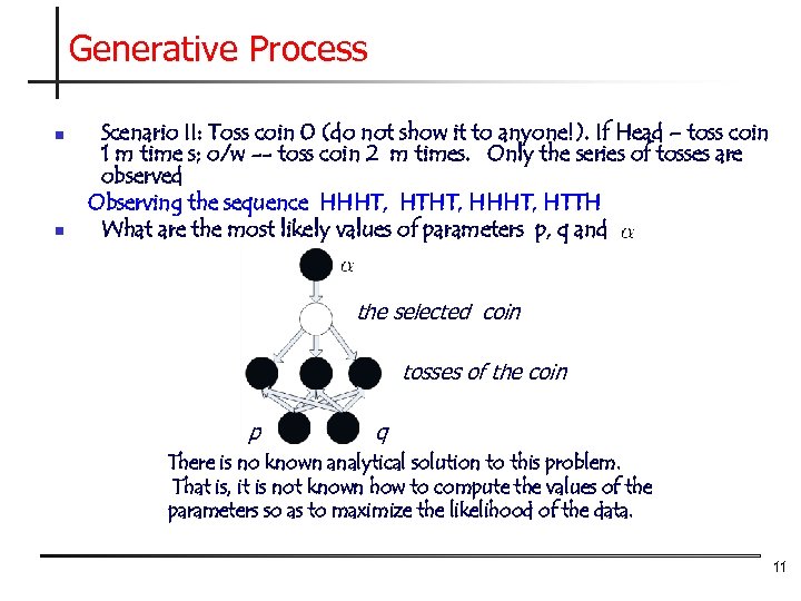Generative Process n n Scenario II: Toss coin 0 (do not show it to anyone!). If Head – toss coin 1 m time s; o/w -- toss coin 2 m times. Only the series of tosses are observed Observing the sequence HHHT, HTHT, HHHT, HTTH What are the most likely values of parameters p, q and the selected coin tosses of the coin p q There is no known analytical solution to this problem. That is, it is not known how to compute the values of the parameters so as to maximize the likelihood of the data. 11

Key Intuition (1) n If we knew which of the data points (HHHT), (HTTH) came from Coin 1 and which from Coin 2, there was no problem. 12

Key Intuition n n n If we knew which of the data points (HHHT), (HTTH) came from Coin 1 and which from Coin 2, there was no problem. Instead, use an iterative approach for estimating the parameters: Guess the probability that a given data point came from Coin 1/2 Generate fictional labels, weighted according to this probability. Now, compute the most likely value of the parameters. [recall NB example] Compute the likelihood of the data given this model. Re-estimate the initial parameter setting: set them to maximize the likelihood of the data. (Labels Model Parameters) Likelihood of the data This process can be iterated and can be shown to converge to a local maximum of the likelihood function 13

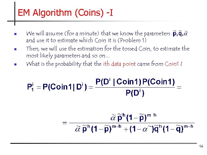EM Algorithm (Coins) -I n n n We will assume (for a minute) that we know the parameters and use it to estimate which Coin it is (Problem 1) Then, we will use the estimation for the tossed Coin, to estimate the most likely parameters and so on. . . What is the probability that the ith data point came from Coin 1 ? 14

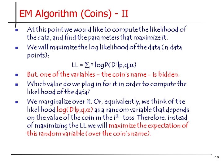EM Algorithm (Coins) - II 15

EM Algorithm (Coins) - III 16

EM Algorithm (Coins) - IV n Explicitly, we get: 17

EM Algorithm (Coins) - V When computing the derivatives, notice here is a constant; it was computed using the current parameters (including ). 18

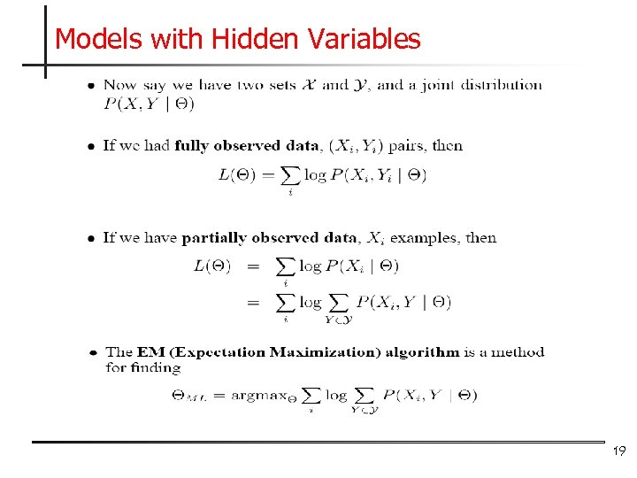Models with Hidden Variables 19

EM 20

EM Summary (so far) n n n EM is a general procedure for learning in the presence of unobserved variables. We have shown how to use it in order to estimate the most likely density function for a mixture of (Bernoulli) distributions. EM is an iterative algorithm that can be shown to converge to a local maximum of the likelihood function. It depends on assuming a family of probability distributions. In this sense, it is a family of algorithms. The update rules you will derive depend on the model assumed. 21