M 248 Analyzing data Block D 1

M 248: Analyzing data Block D 1

Block D UNITS D 3, D 2 Related variables Regression Contents Introduction Section 1: Correlation Section 2: Measures of correlation Section 3: Regression Section 4: Independence (Association in Contingency tables) Terms to know and use 2

Introduction l The slides are based on the following points 1. 2. 3. Correlation between two variables and the strength of this correlation. Regression Studying contingency tables 3

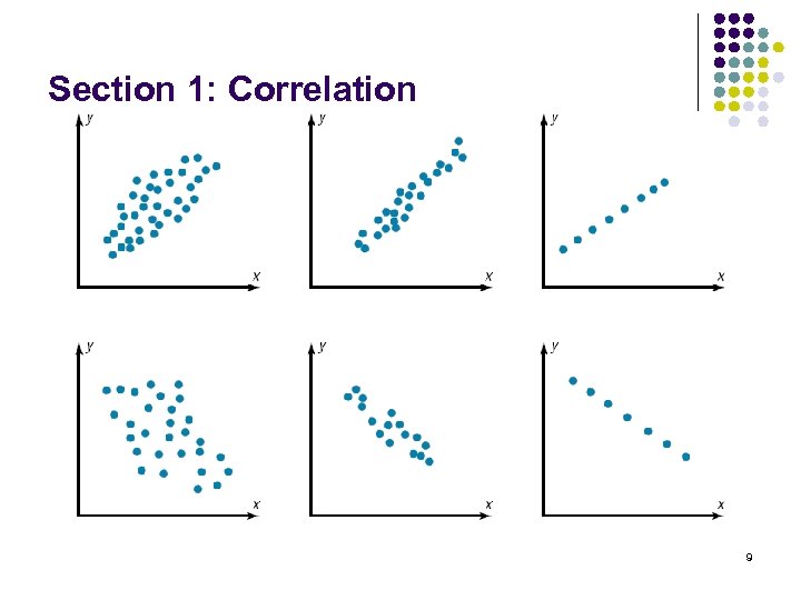
Section 1: Correlation l l Two random variables are said to be related (or correlated or associated) if knowing the value of one variable tells you something about the value of the other. Alternatively we say there is a relationship between the two variables. The first thing to do when investigating a possible relationship between two variables, is to produce a scatterplot of the data. 4

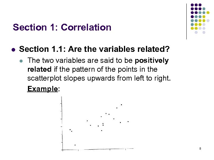
Section 1: Correlation l Section 1. 1: Are the variables related? l The two variables are said to be positively related if the pattern of the points in the scatterplot slopes upwards from left to right. Example: 5

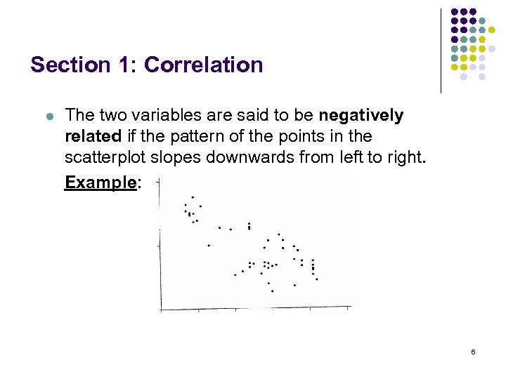
Section 1: Correlation l The two variables are said to be negatively related if the pattern of the points in the scatterplot slopes downwards from left to right. Example: 6

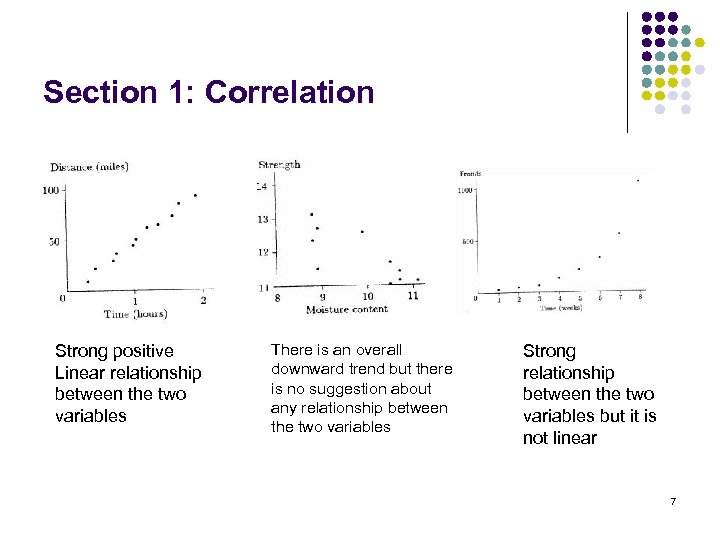
Section 1: Correlation Strong positive Linear relationship between the two variables There is an overall downward trend but there is no suggestion about any relationship between the two variables Strong relationship between the two variables but it is not linear 7

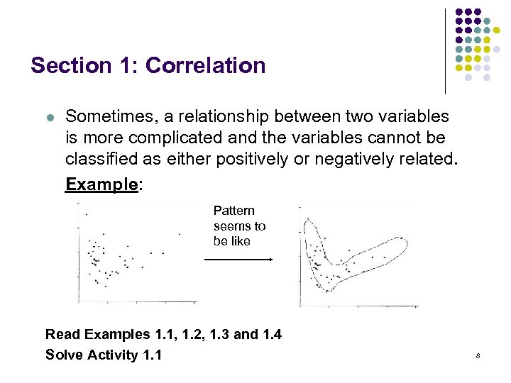
Section 1: Correlation l Sometimes, a relationship between two variables is more complicated and the variables cannot be classified as either positively or negatively related. Example: Pattern seems to be like Read Examples 1. 1, 1. 2, 1. 3 and 1. 4 Solve Activity 1. 1 8

Section 1: Correlation 9

Section 1: Correlation l Section 1. 2: Correlation and Causation and correlation are not equivalent. Causation means that the value of one variable is caused by the value of the other, while correlation means that there is a relationship between the two variables. 10

Section 2: Measures of correlation l l l There are two measures of correlations, The Pearson and the Spearman correlation. These measures are called correlation coefficients. A correlation coefficient is a number between -1 and +1, the closer it is of those limits, the stronger the relationship between the two variables. Correlation coefficients which measure how well a straight line can explain the relationship between two variables are called linear correlation coefficients. 11

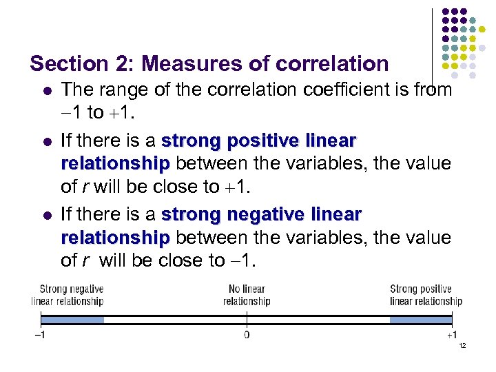
Section 2: Measures of correlation l l l The range of the correlation coefficient is from 1 to 1. If there is a strong positive linear relationship between the variables, the value of r will be close to 1. If there is a strong negative linear relationship between the variables, the value of r will be close to 1. 12

Section 2: Measures of correlation l Section 2. 1: The Pearson correlation coefficient Two variables are said to be positively related if they increase together and decrease together, then the correlation coefficient will be positive. And if they are negatively related then it will be negative. A correlation coefficient of 0 implies that there is no systematic linear relationship between the two variables. 13

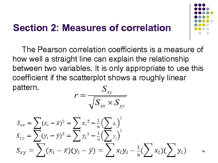
Section 2: Measures of correlation The Pearson correlation coefficients is a measure of how well a straight line can explain the relationship between two variables. It is only appropriate to use this coefficient if the scatterplot shows a roughly linear pattern. 14

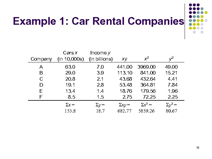
Example 1: Car Rental Companies Company Cars x (in 10, 000 s) Income y (in billions) xy x 2 y 2 A B C D E F 63. 0 29. 0 20. 8 19. 1 13. 4 8. 5 7. 0 3. 9 2. 1 2. 8 1. 4 1. 5 441. 00 113. 10 43. 68 53. 48 18. 76 2. 75 3969. 00 841. 00 432. 64 364. 81 179. 56 72. 25 49. 00 15. 21 4. 41 7. 84 1. 96 2. 25 Σx = 153. 8 Σy = 18. 7 Σxy = 682. 77 Σx 2 = 5859. 26 Σy 2 = 80. 67 15

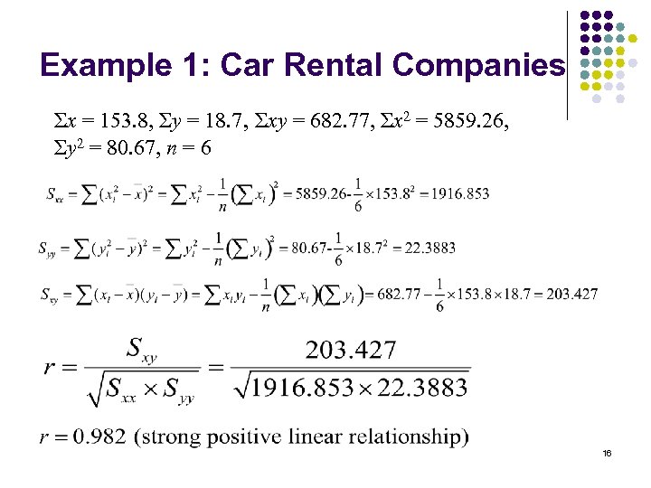
Example 1: Car Rental Companies Σx = 153. 8, Σy = 18. 7, Σxy = 682. 77, Σx 2 = 5859. 26, Σy 2 = 80. 67, n = 6 16

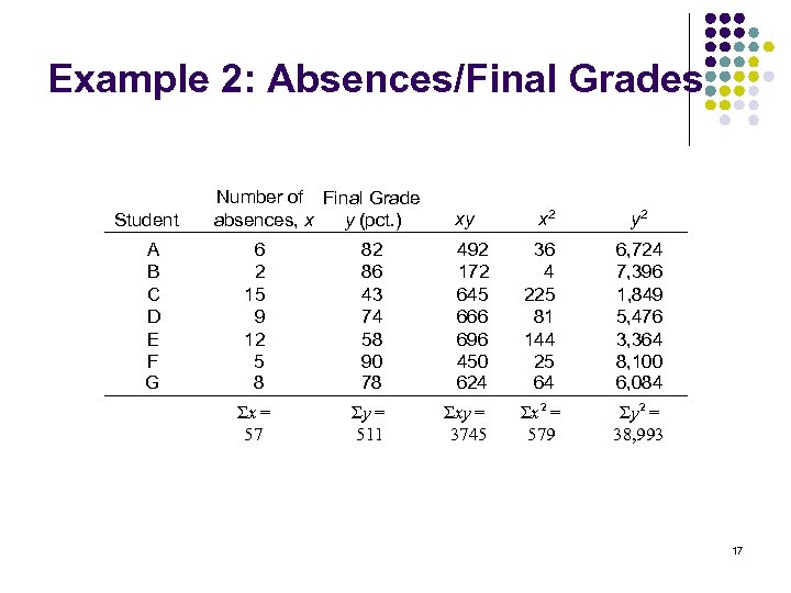
Example 2: Absences/Final Grades Student A B C D E F G Number of Final Grade absences, x y (pct. ) xy 6 2 15 9 12 5 8 82 86 43 74 58 90 78 492 172 645 666 696 450 624 Σx = 57 Σy = 511 Σxy = 3745 x 2 36 4 225 81 144 25 64 Σx 2 = 579 y 2 6, 724 7, 396 1, 849 5, 476 3, 364 8, 100 6, 084 Σy 2 = 38, 993 17

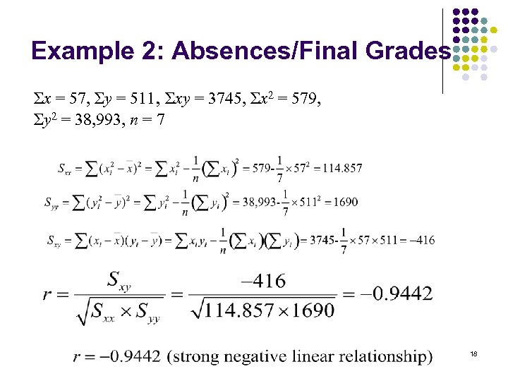
Example 2: Absences/Final Grades Σx = 57, Σy = 511, Σxy = 3745, Σx 2 = 579, Σy 2 = 38, 993, n = 7 18

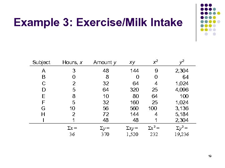
Example 3: Exercise/Milk Intake Subject A B C D E F G H I Hours, x Amount y xy 3 0 2 5 8 5 10 2 1 Σx = 36 48 8 32 64 10 32 56 72 48 Σy = 370 144 0 64 320 80 160 560 144 48 Σxy = 1, 520 x 2 9 0 4 25 64 25 100 4 1 Σx 2 = 232 y 2 2, 304 64 1, 024 4, 096 100 1, 024 3, 136 5, 184 2, 304 Σy 2 = 19, 236 19

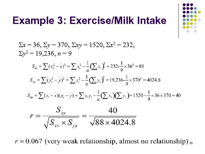
Example 3: Exercise/Milk Intake Σx = 36, Σy = 370, Σxy = 1520, Σx 2 = 232, Σy 2 = 19, 236, n = 9 20

Section 2: Measures of correlation Section 2. 2: The Spearman rank correlation coefficient Replacing the original data by their ranks, and measuring the strength of association between two variables by calculating the Pearson correlation coefficient with the ranks is known as the Spearman rank correlation coefficient, and is denoted by rs The values of rs is a measure of the linearity of the relationship between the ranks. l 21

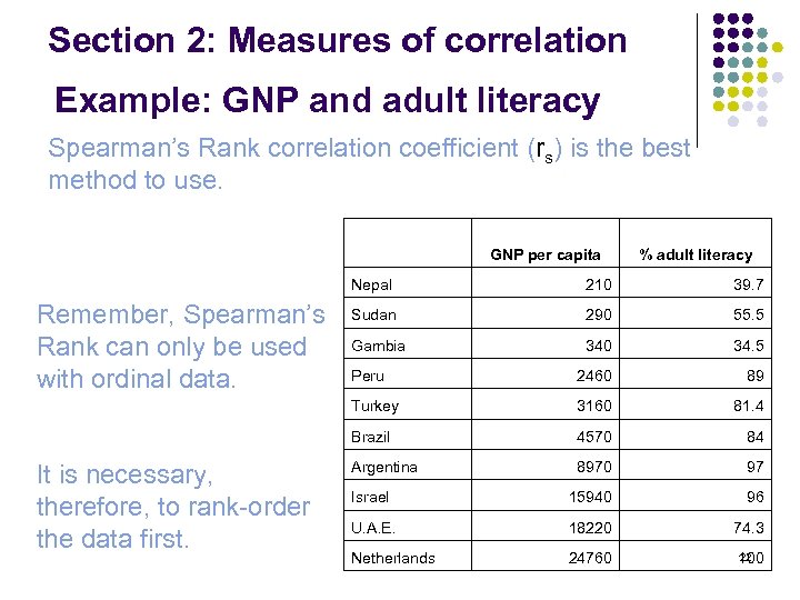
Section 2: Measures of correlation Example: GNP and adult literacy Spearman’s Rank correlation coefficient (rs) is the best method to use. GNP per capita % adult literacy Nepal Sudan 290 55. 5 Gambia 340 34. 5 Peru 2460 89 3160 81. 4 Brazil It is necessary, therefore, to rank-order the data first. 39. 7 Turkey Remember, Spearman’s Rank can only be used with ordinal data. 210 4570 84 Argentina 8970 97 Israel 15940 96 U. A. E. 18220 74. 3 Netherlands 24760 22 100

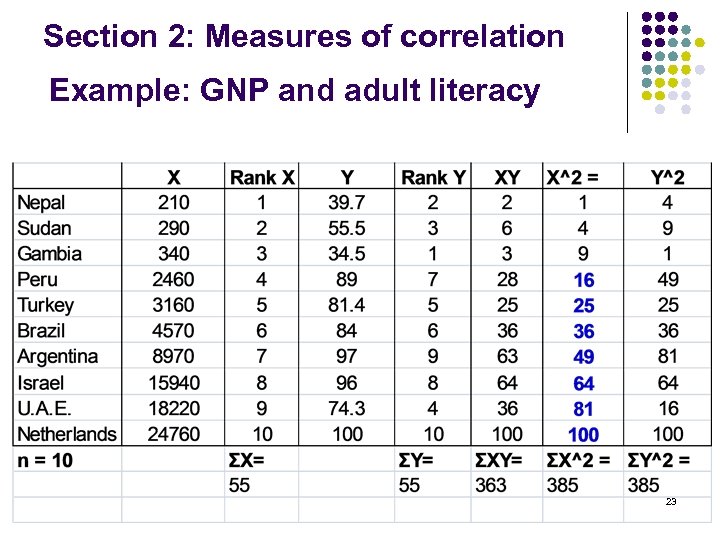
Section 2: Measures of correlation Example: GNP and adult literacy 23

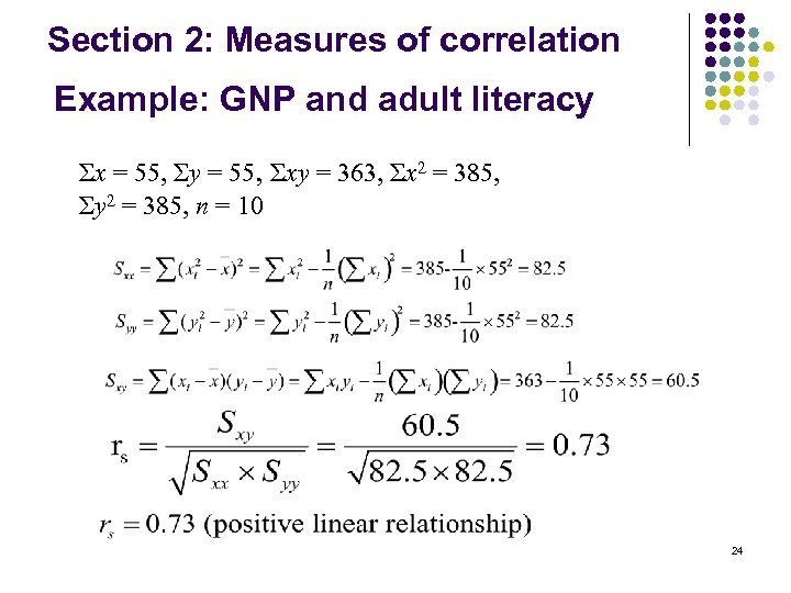
Section 2: Measures of correlation Example: GNP and adult literacy Σx = 55, Σy = 55, Σxy = 363, Σx 2 = 385, Σy 2 = 385, n = 10 24

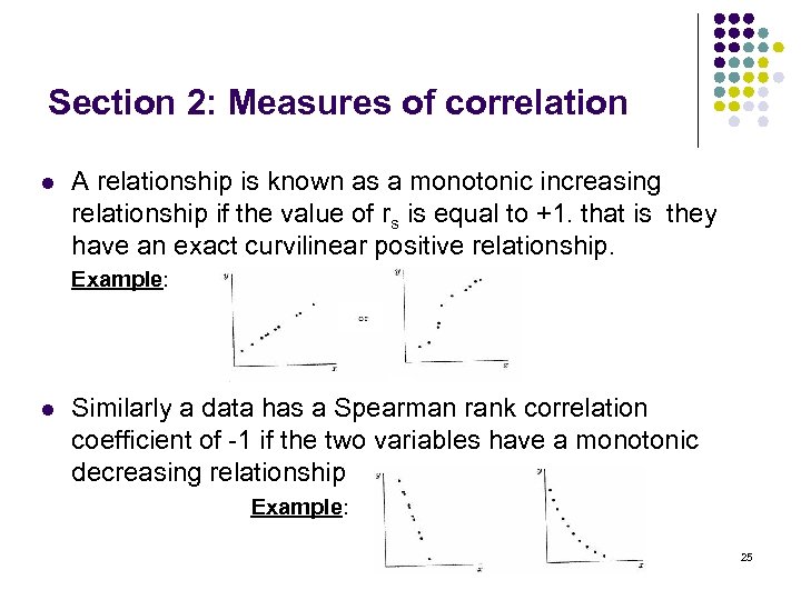
Section 2: Measures of correlation l A relationship is known as a monotonic increasing relationship if the value of rs is equal to +1. that is they have an exact curvilinear positive relationship. Example: l Similarly a data has a Spearman rank correlation coefficient of -1 if the two variables have a monotonic decreasing relationship Example: 25

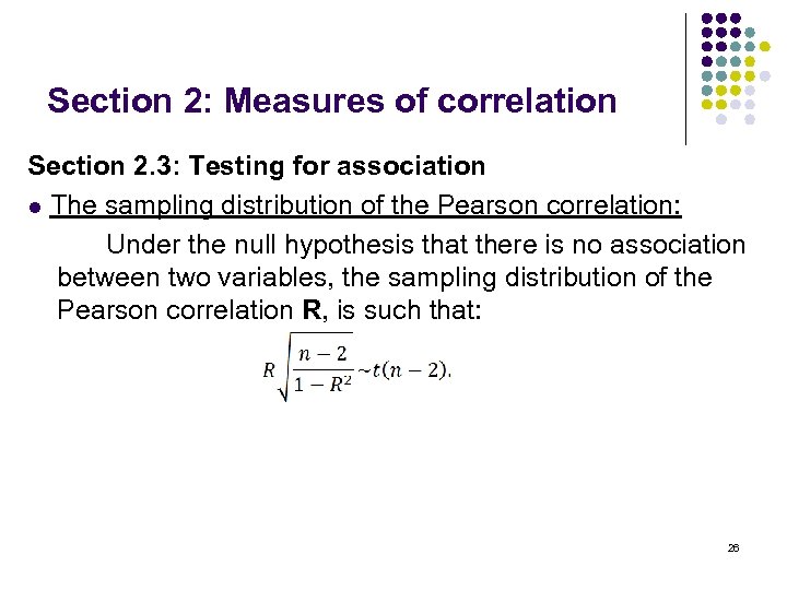
Section 2: Measures of correlation Section 2. 3: Testing for association l The sampling distribution of the Pearson correlation: Under the null hypothesis that there is no association between two variables, the sampling distribution of the Pearson correlation R, is such that: 26

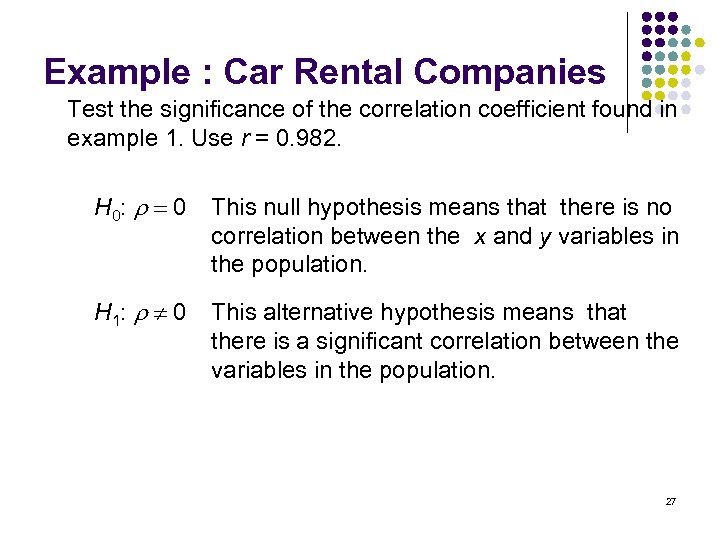
Example : Car Rental Companies Test the significance of the correlation coefficient found in example 1. Use r = 0. 982. H 0: 0 This null hypothesis means that there is no correlation between the x and y variables in the population. H 1: 0 This alternative hypothesis means that there is a significant correlation between the variables in the population. 27

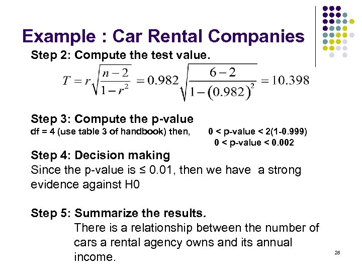
Example : Car Rental Companies Step 2: Compute the test value. Step 3: Compute the p-value df = 4 (use table 3 of handbook) then, 0 < p-value < 2(1 -0. 999) 0 < p-value < 0. 002 Step 4: Decision making Since the p-value is ≤ 0. 01, then we have a strong evidence against H 0 Step 5: Summarize the results. There is a relationship between the number of cars a rental agency owns and its annual income. 28

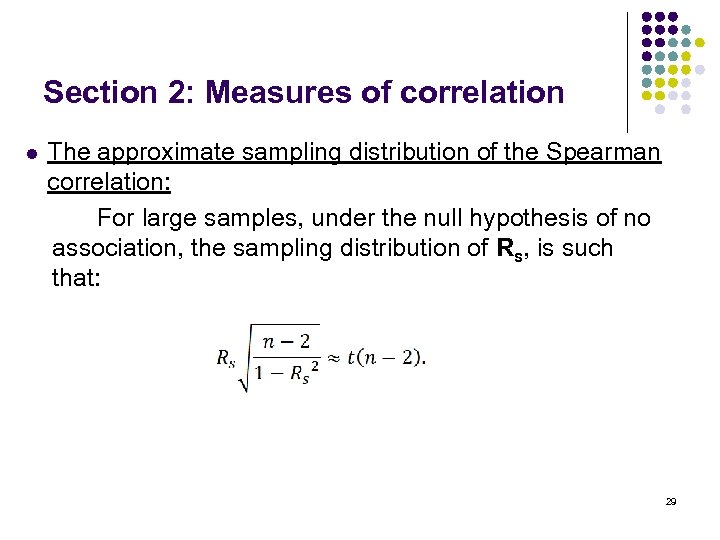
Section 2: Measures of correlation l The approximate sampling distribution of the Spearman correlation: For large samples, under the null hypothesis of no association, the sampling distribution of Rs, is such that: 29

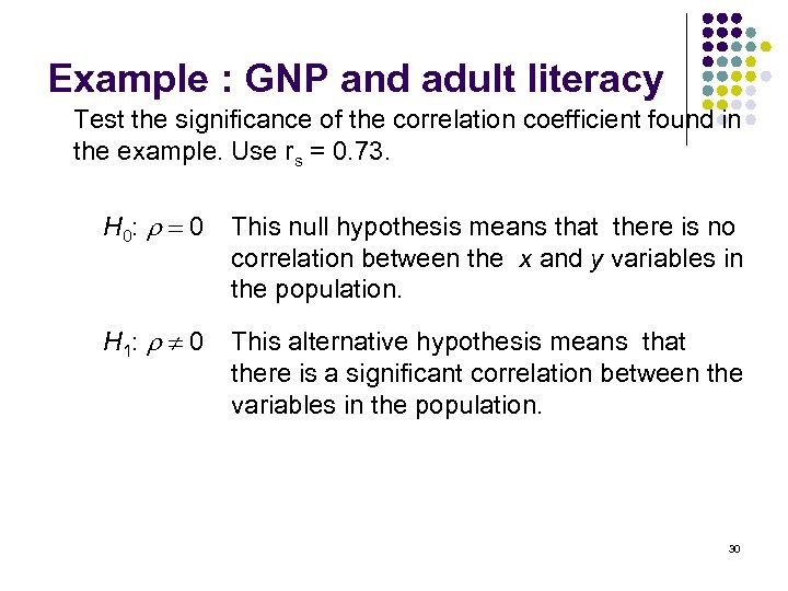
Example : GNP and adult literacy Test the significance of the correlation coefficient found in the example. Use rs = 0. 73. H 0: 0 This null hypothesis means that there is no correlation between the x and y variables in the population. H 1: 0 This alternative hypothesis means that there is a significant correlation between the variables in the population. 30

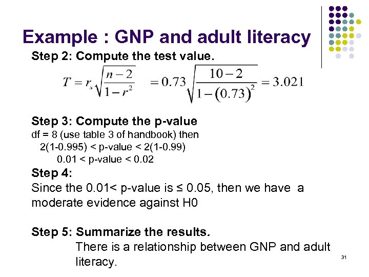
Example : GNP and adult literacy Step 2: Compute the test value. Step 3: Compute the p-value df = 8 (use table 3 of handbook) then 2(1 -0. 995) < p-value < 2(1 -0. 99) 0. 01 < p-value < 0. 02 Step 4: Since the 0. 01< p-value is ≤ 0. 05, then we have a moderate evidence against H 0 Step 5: Summarize the results. There is a relationship between GNP and adult literacy. 31

Section 2: Measures of correlation l Section 2. 4: Correlation using MINITAB See MINITAB Videos on moodle 32

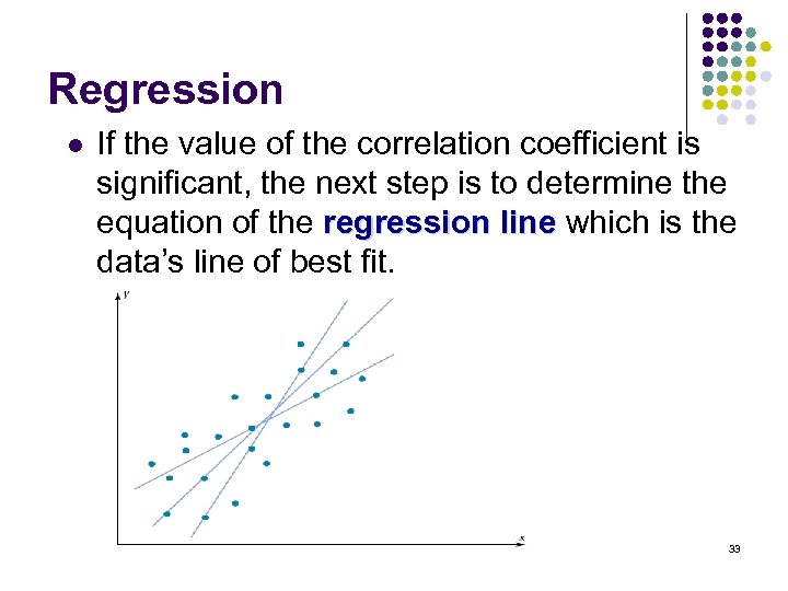
Regression l If the value of the correlation coefficient is significant, the next step is to determine the equation of the regression line which is the data’s line of best fit. 33

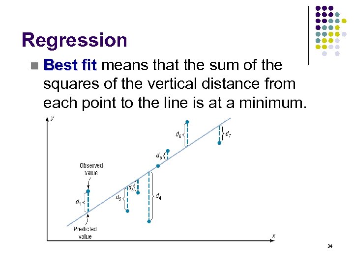
Regression n Best fit means that the sum of the squares of the vertical distance from each point to the line is at a minimum. 34

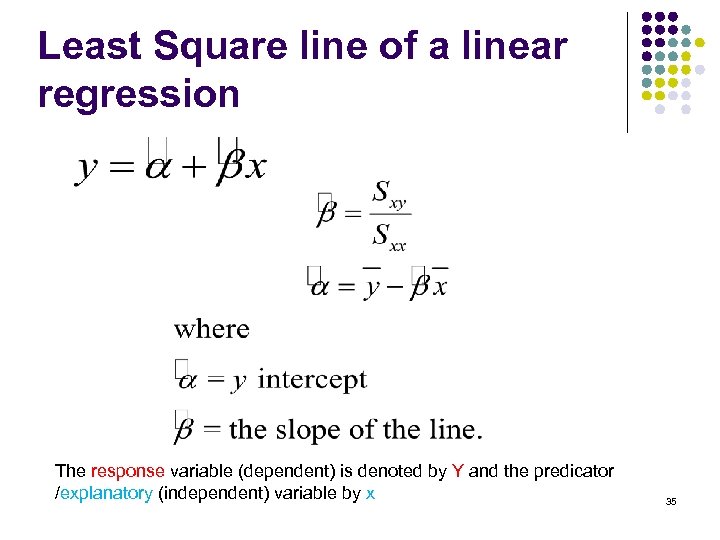
Least Square line of a linear regression The response variable (dependent) is denoted by Y and the predicator /explanatory (independent) variable by x 35

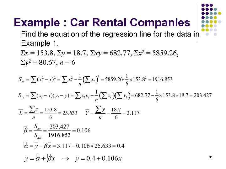
Example : Car Rental Companies Find the equation of the regression line for the data in Example 1. Σx = 153. 8, Σy = 18. 7, Σxy = 682. 77, Σx 2 = 5859. 26, Σy 2 = 80. 67, n = 6 36

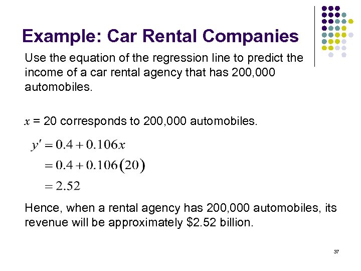
Example: Car Rental Companies Use the equation of the regression line to predict the income of a car rental agency that has 200, 000 automobiles. x = 20 corresponds to 200, 000 automobiles. Hence, when a rental agency has 200, 000 automobiles, its revenue will be approximately $2. 52 billion. 37

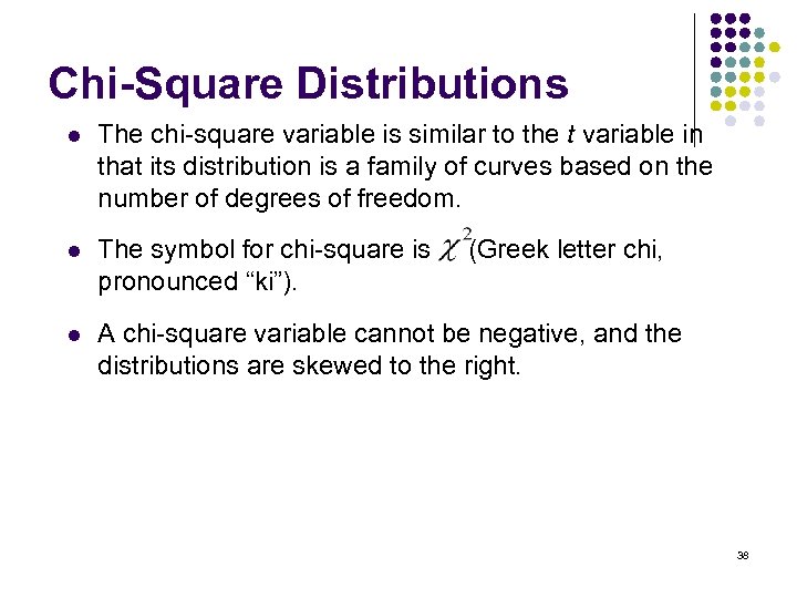
Chi-Square Distributions l The chi-square variable is similar to the t variable in that its distribution is a family of curves based on the number of degrees of freedom. l The symbol for chi-square is (Greek letter chi, pronounced “ki”). l A chi-square variable cannot be negative, and the distributions are skewed to the right. 38

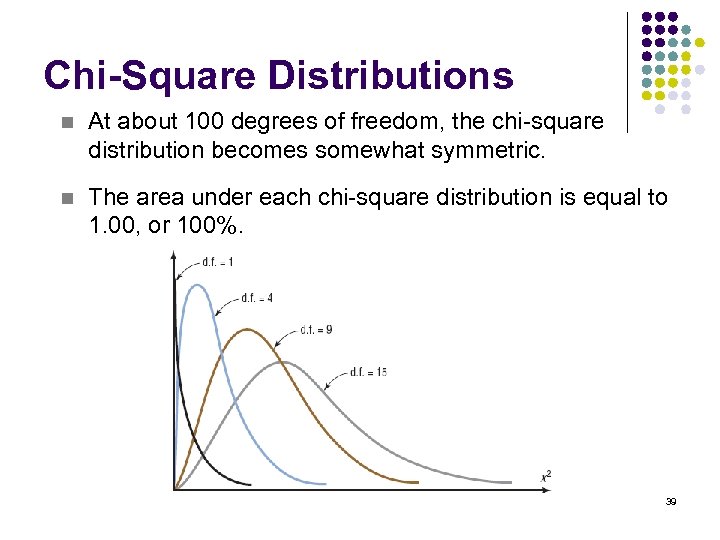
Chi-Square Distributions n At about 100 degrees of freedom, the chi-square distribution becomes somewhat symmetric. n The area under each chi-square distribution is equal to 1. 00, or 100%. 39

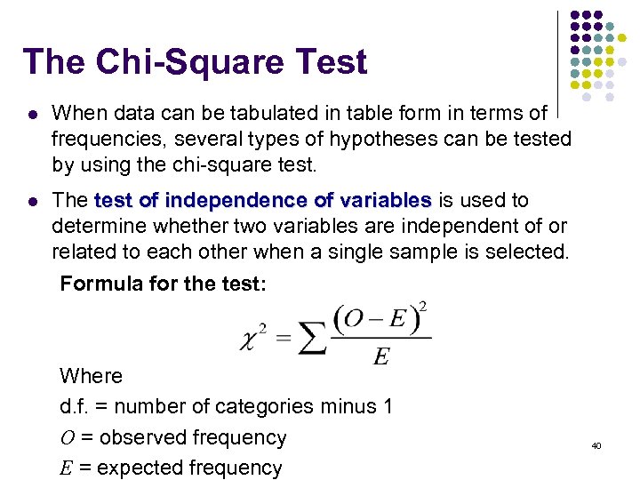
The Chi-Square Test l When data can be tabulated in table form in terms of frequencies, several types of hypotheses can be tested by using the chi-square test. l The test of independence of variables is used to determine whether two variables are independent of or related to each other when a single sample is selected. Formula for the test: Where d. f. = number of categories minus 1 O = observed frequency E = expected frequency 40

Test for Independence l l The chi-square test can be used to test the independence of two variables. The hypotheses are: l H 0: There is no relationship between two variables. l H 1: There is a relationship between two variables. If the null hypothesis is rejected, there is some relationship between the variables. In order to test the null hypothesis, one must compute the expected frequencies, assuming the null hypothesis is true. 41

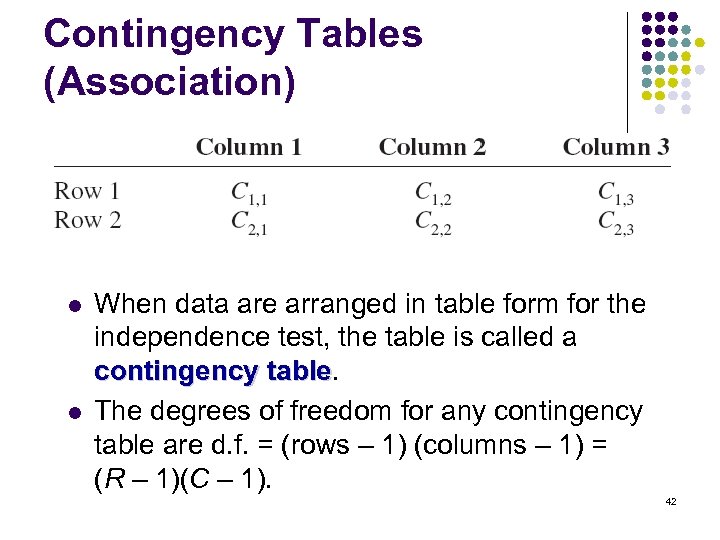
Contingency Tables (Association) l l When data are arranged in table form for the independence test, the table is called a contingency table The degrees of freedom for any contingency table are d. f. = (rows – 1) (columns – 1) = (R – 1)(C – 1). 42

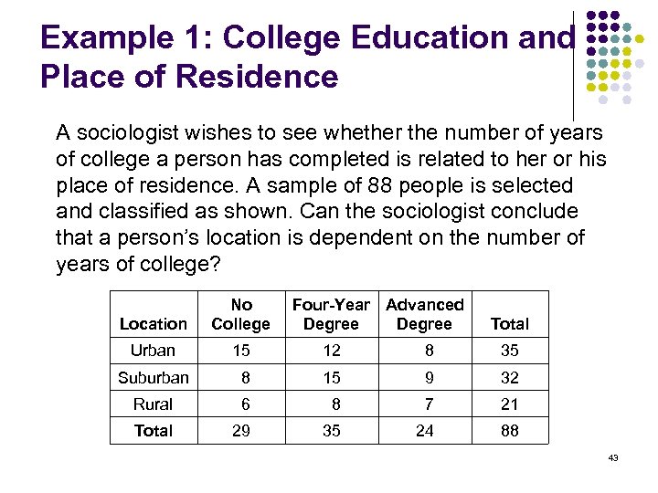
Example 1: College Education and Place of Residence A sociologist wishes to see whether the number of years of college a person has completed is related to her or his place of residence. A sample of 88 people is selected and classified as shown. Can the sociologist conclude that a person’s location is dependent on the number of years of college? Location No College Four-Year Advanced Degree Urban 15 12 8 35 Suburban 8 15 9 32 Rural 6 8 7 21 Total 29 35 24 88 Total 43

Example 1: College Education and Place of Residence Step 1: State the hypotheses and identify the claim. H 0: A person’s place of residence is independent of the number of years of college completed. H 1: A person’s place of residence is dependent on the number of years of college completed (claim). 44

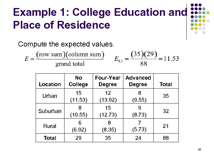
Example 1: College Education and Place of Residence Compute the expected values. Location No College Four-Year Advanced Degree Total Urban 15 (11. 53) 12 (13. 92) 8 (9. 55) 35 Suburban 8 (10. 55) 15 (12. 73) 9 (8. 73) 32 Rural 6 (6. 92) 8 (8. 35) 7 (5. 73) 21 Total 29 35 24 88 45

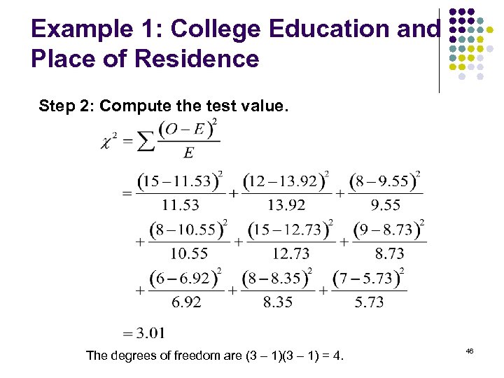
Example 1: College Education and Place of Residence Step 2: Compute the test value. The degrees of freedom are (3 – 1) = 4. 46

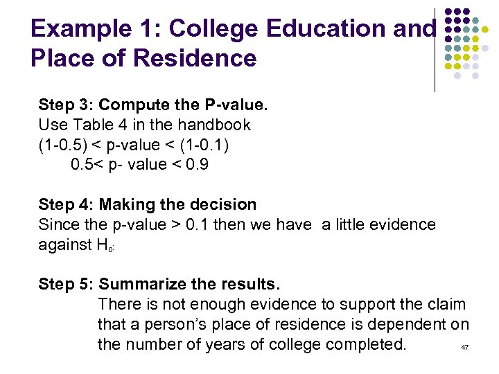
Example 1: College Education and Place of Residence Step 3: Compute the P-value. Use Table 4 in the handbook (1 -0. 5) < p-value < (1 -0. 1) 0. 5< p- value < 0. 9 Step 4: Making the decision Since the p-value > 0. 1 then we have a little evidence against H : 0 Step 5: Summarize the results. There is not enough evidence to support the claim that a person’s place of residence is dependent on the number of years of college completed. 47

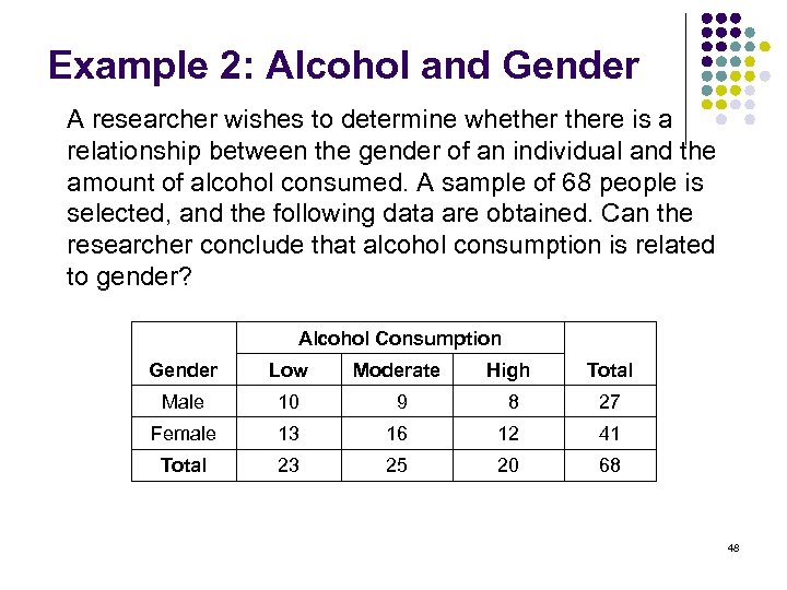
Example 2: Alcohol and Gender A researcher wishes to determine whethere is a relationship between the gender of an individual and the amount of alcohol consumed. A sample of 68 people is selected, and the following data are obtained. Can the researcher conclude that alcohol consumption is related to gender? Alcohol Consumption Gender Low Moderate High Total Male 10 9 8 27 Female 13 16 12 41 Total 23 25 20 68 48

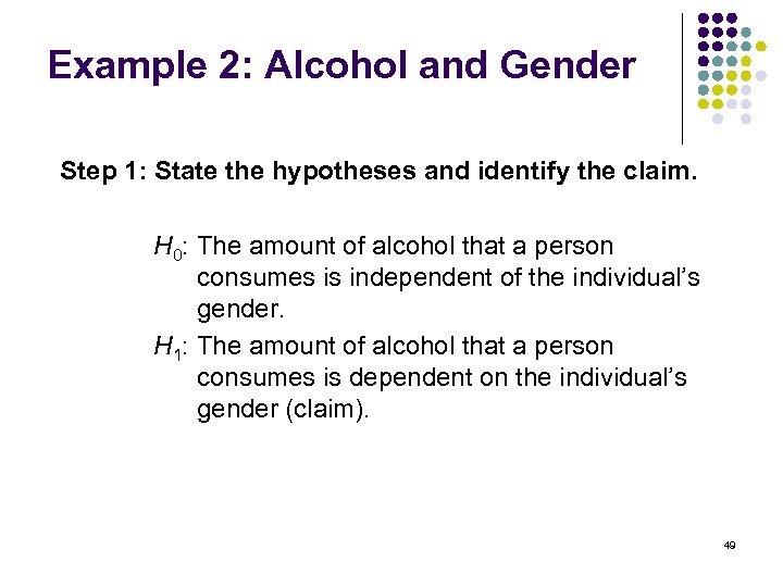
Example 2: Alcohol and Gender Step 1: State the hypotheses and identify the claim. H 0: The amount of alcohol that a person consumes is independent of the individual’s gender. H 1: The amount of alcohol that a person consumes is dependent on the individual’s gender (claim). 49

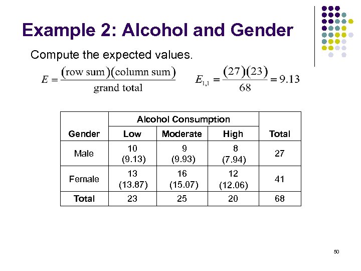
Example 2: Alcohol and Gender Compute the expected values. Alcohol Consumption Gender Low Moderate High Total Male 10 (9. 13) 9 (9. 93) 8 (7. 94) 27 Female 13 (13. 87) 16 (15. 07) 12 (12. 06) 41 Total 23 25 20 68 50

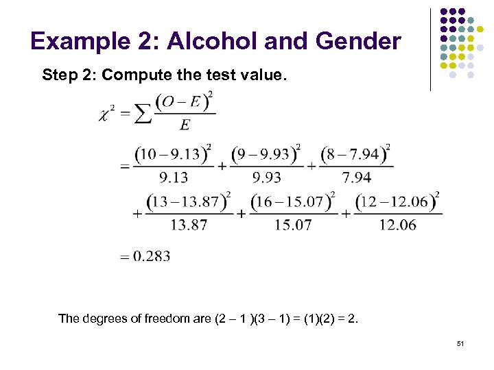
Example 2: Alcohol and Gender Step 2: Compute the test value. The degrees of freedom are (2 – 1 )(3 – 1) = (1)(2) = 2. 51

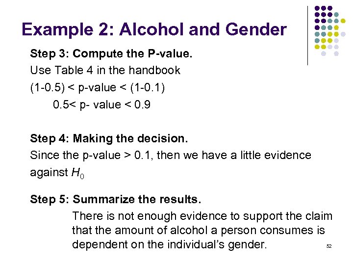
Example 2: Alcohol and Gender Step 3: Compute the P-value. Use Table 4 in the handbook (1 -0. 5) < p-value < (1 -0. 1) 0. 5< p- value < 0. 9 Step 4: Making the decision. Since the p-value > 0. 1, then we have a little evidence against H 0 Step 5: Summarize the results. There is not enough evidence to support the claim that the amount of alcohol a person consumes is 52 dependent on the individual’s gender.

Terms to know and use l l l l Related variable Correlation Association Causation Positively related Negatively related Monotonic increasing Monotonic decreasing l l Monotonic relationship Correlation coefficient Pearson correlation coefficient Spearman rank correlation coefficient 53

Terms to know and use l l l Explanatory variables Response variable Linear regression model Regression line Least square line Contingency Table l l Independence Association 54