Longitudinal Data Analysis for Social Science Researchers Research

Longitudinal Data Analysis for Social Science Researchers Research Value of Longitudinal Data www. longitudinal. stir. ac. uk

Longitudinal Data – Time Series – Macro Level Data that tends to consist of one or a few variables commonly measured on just one or a few cases (e. g. a country or the EU states) on at least ten occasions. - Unemployment rates, RPI, Share Prices

Longitudinal Studies – Micro Level Longitudinal studies in the social sciences tend to consist of • many cases (usually thousands) • large number of variables • fewer occasions (e. g. household contacted yearly)

A Panel A particular set of respondents are questioned (or measured) repeatedly. The great sociologist Paul H. Lazarsfeld coined this term.

A Cohort Study Cohort studies are concerned with charting the development of groups from a particular time point. A special form of panel study in my view.

Two main examples of types of cohort studies • Age Cohort - defined by an age group. [Youth Cohort Study of England & Wales] [qualified nurses survey] [retirement study] • Birth Cohorts - people born at a certain time. [1946, 1958 & 1970 birth cohorts; Millennium]

STUDY DESIGNS

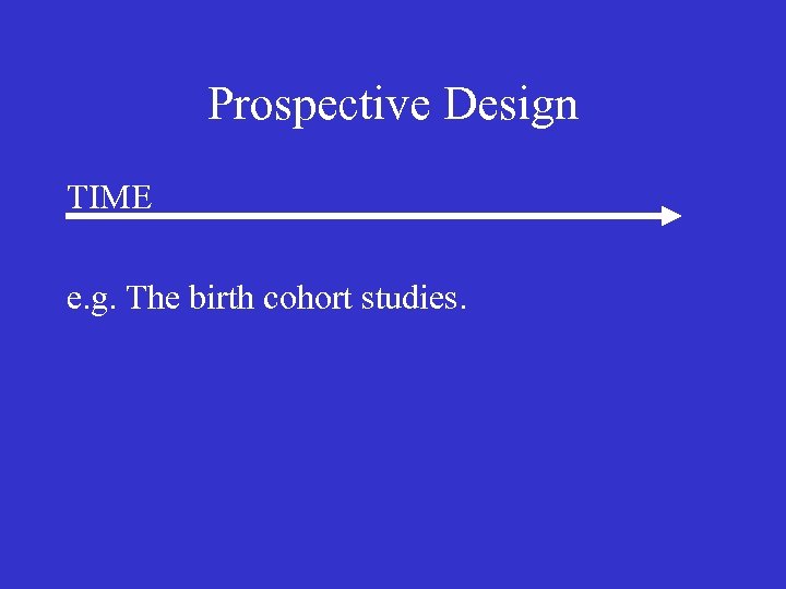Prospective Design TIME e. g. The birth cohort studies.

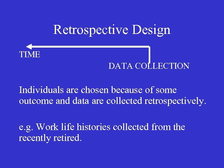Retrospective Design TIME DATA COLLECTION Individuals are chosen because of some outcome and data are collected retrospectively. e. g. Work life histories collected from the recently retired.

Mixed Retrospective and Prospective Design 10 year olds might be chosen as part of a retrospective study and then followed prospectively until they reach the end of compulsory education.

PROSPECTIVE OR RETROSPECTIVE? SOME ISSUES TO CONSIDER • Length of time from an event is an important issue • Recall – how much did you weigh at age 13? • Remember the first and last time you had sex • Telescoping of time – how long did you stay in your second job?

SOME MORE ISSUES TO CONSIDER • The search for meaning – why did you leave your job in 1970? • Attitudes and values are hard to disentangle from events • Emotions for example are temporal (e. g. anxiety before surgery) • Under-reporting of undesirable events • Over-reporting of desirable events

SOME METHODOLOGICAL ISSUES

Davies, R. B. (1994) ‘From Cross-Sectional to Longitudinal Analysis’ in Dale A. and Davies, R. B. Analyzing Social & Political Change, Sage.

A glib claim that longitudinal data analysis is important because it permits insights into the processes of change is inadequate and certainly fails to convince many social science researchers who are concerned with substantive rather than methodological challenges. What is required is an understanding on the limitations of crosssectional analysis.

Four Methodological Issues • • Age, Cohort & Period Effects Direction of Causality State Dependence Residual Heterogeneity

Age, Cohort, Period • AGE = Amount of time since cohort was constituted. • COHORT = A common group being studied. • PERIOD = Moment of observation.

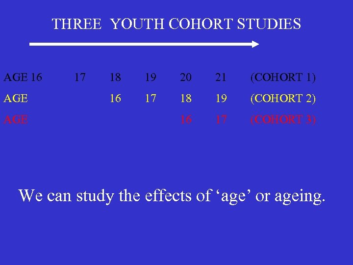THREE YOUTH COHORT STUDIES AGE 16 AGE 17 18 19 20 21 (COHORT 1) 16 17 18 19 (COHORT 2) 16 17 (COHORT 3) We can study the effects of ‘age’ or ageing.

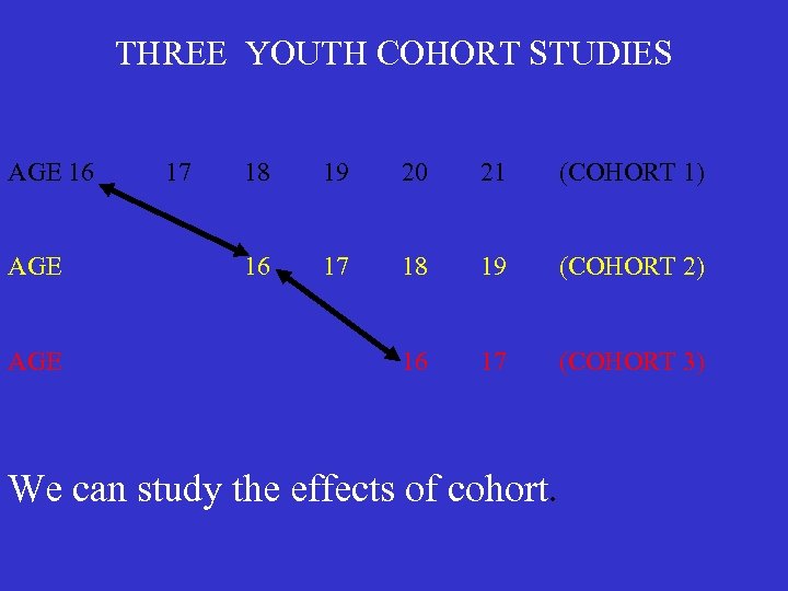THREE YOUTH COHORT STUDIES AGE 16 AGE 17 18 19 20 21 (COHORT 1) 16 17 18 19 (COHORT 2) 16 17 (COHORT 3) We can study the effects of cohort.

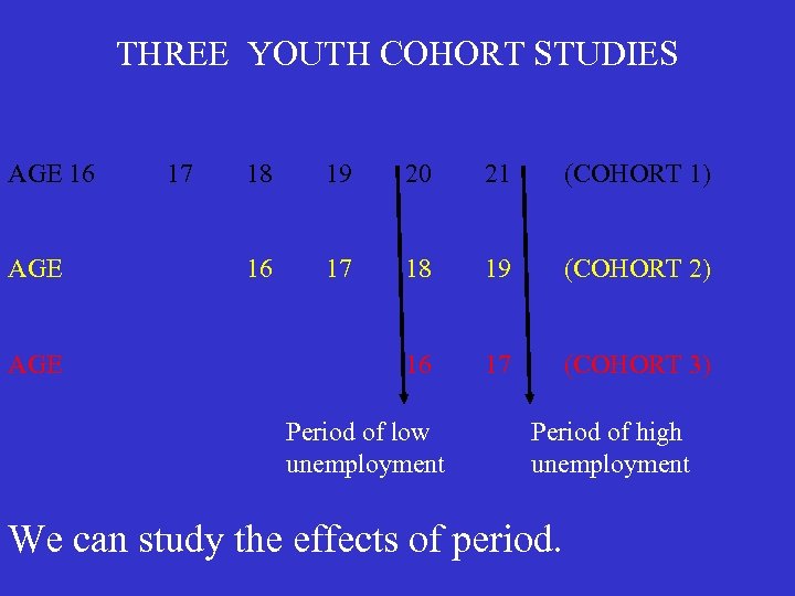THREE YOUTH COHORT STUDIES AGE 16 AGE 17 18 19 20 21 (COHORT 1) 16 17 18 19 (COHORT 2) 16 17 (COHORT 3) Period of low unemployment Period of high unemployment We can study the effects of period.

Pooling cross-sectional datasets can help us begin to unravel period and cohort effects. In most cased even with pooled crosssectional data it is still not conceptually straightforward to disentangle the effects of ageing from period and cohort effects.

Simple Example… Comparing the longitudinal data of three birth cohort studies would facilitate a more thorough analysis of age/cohort/period effects.

Beware: The textbooks tell us that panel data will help use disentangle age/cohort/period effects. In practice however, even with panel data it may still not be possible to clearly disentangle theses effects. Whilst conceptually it is plausible, in our experience, in practice it is difficult to estimate models that clearly disentangle all three effects.

Direction of Causality There is unequivocal evidence from crosssectional data that, overall, the unemployed have poorer health.

This is consistent with both a) unemployment causing ill health and b) ill health causing unemployment

If we had a cross-sectional survey that asked how long people had been unemployed and also their level of health, generally, we would find a negative relationship.

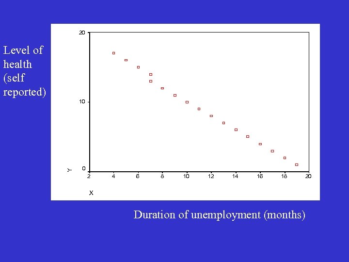20 Level of health (self reported) Y 10 0 2 4 6 8 10 12 14 16 18 X Duration of unemployment (months) 20

Negative – Lower levels of health for people who had been unemployed for longer.

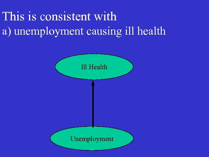This is consistent with a) unemployment causing ill health Ill Health Unemployment

HOWEVER………….

If ill health causes unemployment… then people with comparatively modest levels of ill health will tend to recover more quickly and return to work.

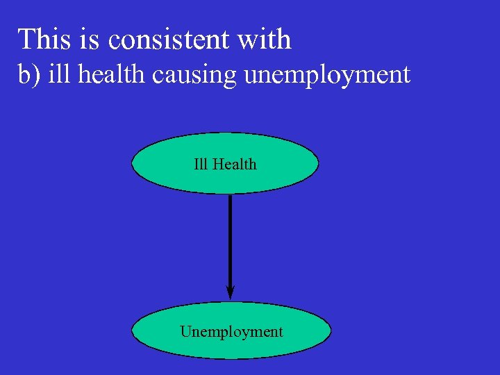This is consistent with b) ill health causing unemployment Ill Health Unemployment

With the increasing duration of unemployment those with less severe ill health will be progressively under represented while those with more severe ill health will be over represented.

This is known as a‘sample selection bias’ and could therefore explain the crosssectional picture of declining ill health with duration of unemployment.

It is not possible to untangle this conundrum with cross-sectional data. Longitudinal data are required!

Month Level of Health Employ Status 1 2 3 4 5 6 7 8 9 10 11 12 17 17 17 10 16 5 4 3 2 1 Employed Unemployed Unemployed Unemployed

Person A Became unemployed and this has affected their level of health.

Month Level of Health Employ Status 1 2 3 4 5 6 7 8 9 10 11 12 17 1 1 1 Employed Unemployed Unemployed Unemployed

Person B Ill health has led to unemployment (because of poor performance).

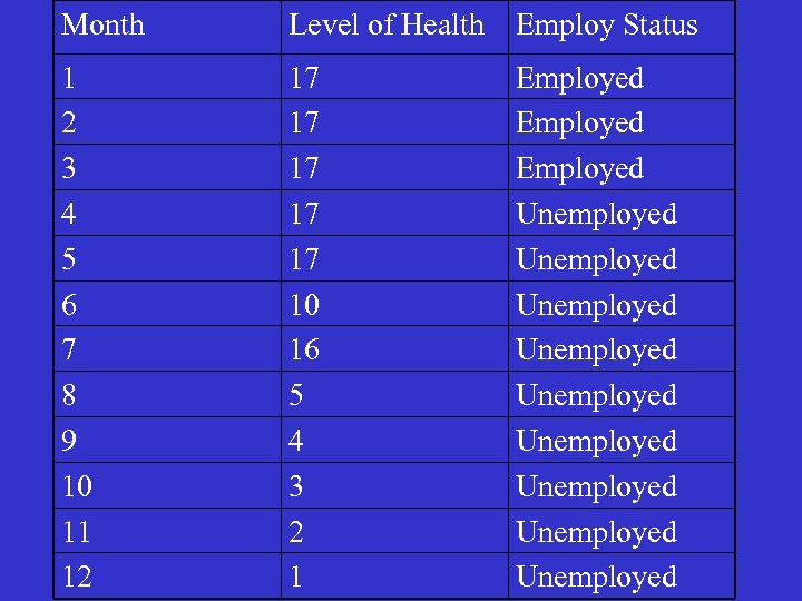Month Level of Health Employ Status 1 2 3 4 5 6 7 8 9 10 11 12 17 17 17 10 16 5 4 3 2 1 Employed Unemployed Unemployed Unemployed

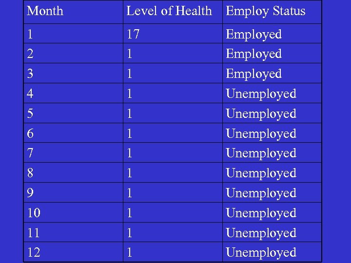Month Level of Health Employ Status 1 2 3 4 5 6 7 8 9 10 11 12 17 1 1 1 Employed Unemployed Unemployed Unemployed

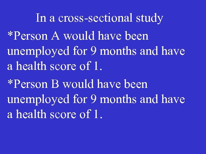In a cross-sectional study *Person A would have been unemployed for 9 months and have a health score of 1. *Person B would have been unemployed for 9 months and have a health score of 1.

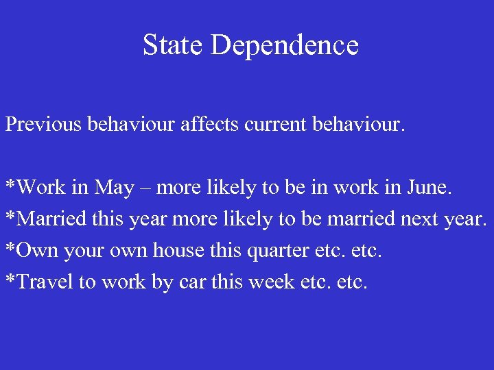State Dependence Previous behaviour affects current behaviour. *Work in May – more likely to be in work in June. *Married this year more likely to be married next year. *Own your own house this quarter etc. *Travel to work by car this week etc.

Residual Heterogeneity (Omitted Explanatory Variables) (Unobserved Heterogeneity)

The possibility of substantial variation between similar individuals due to unmeasured and possibly unmeasureable variables is known as ‘residual heterogeneity’.

There is no way of accounting for omitted explanatory variables in crosssectional analysis. As long as we make the assumption that (at least some of) these effects are enduring there are techniques for accounting for omitted explanatory variables if we have data at more than one time point.

Because data collection instruments often fail to capture the detailed nature of social life there is, almost inevitably, considerable heterogeneity in response variables even amongst respondents that share the same characteristics across all of the explanatory variables.

It is sometimes claimed that the main advantage of longitudinal data is that it facilitates improved control for the plethora of variables that are omitted from any analysis.

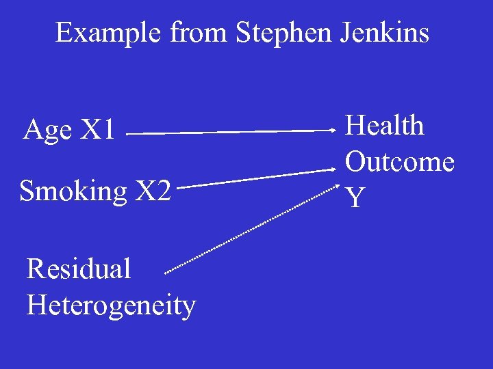Example from Stephen Jenkins Age X 1 Smoking X 2 Residual Heterogeneity Health Outcome Y

The residual heterogeneity is an “unmeasured” or even “unmeasureable” variable

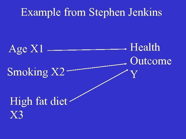Example from Stephen Jenkins Age X 1 Smoking X 2 High fat diet X 3 Health Outcome Y

Another Example Consider a very simple example of a study unemployment.

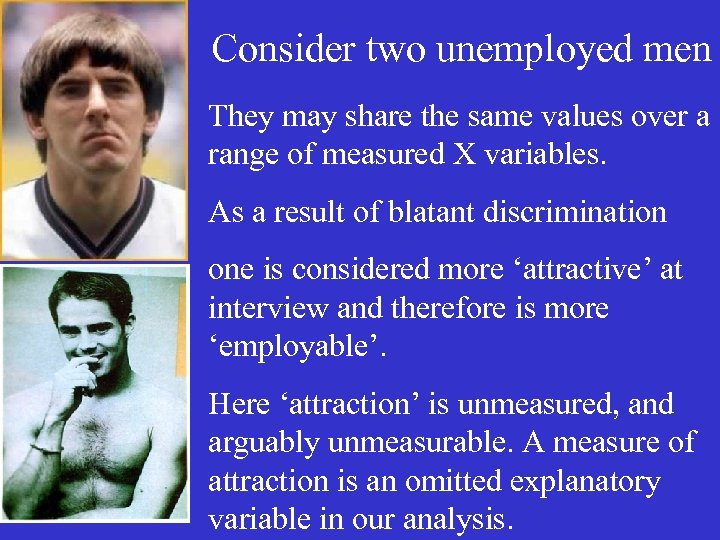Consider two unemployed men They may share the same values over a range of measured X variables. As a result of blatant discrimination one is considered more ‘attractive’ at interview and therefore is more ‘employable’. Here ‘attraction’ is unmeasured, and arguably unmeasurable. A measure of attraction is an omitted explanatory variable in our analysis.

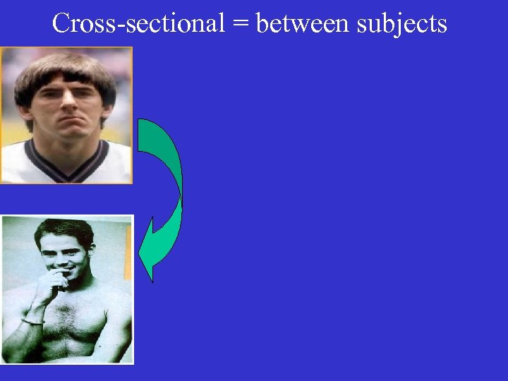Cross-sectional = between subjects

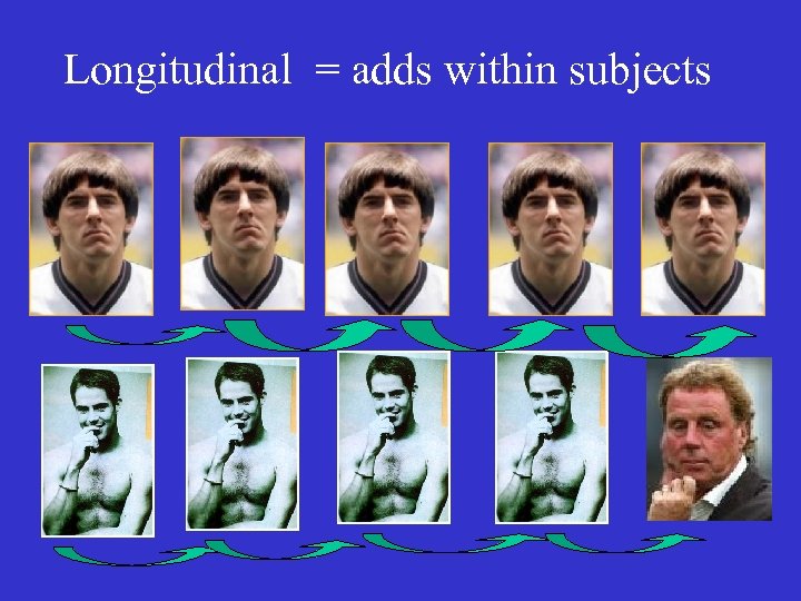Longitudinal = adds within subjects

Residual Heterogeneity (Omitted Explanatory Variables) (Unobserved Heterogeneity) • Panel data are an improvement on cross-sectional • Panel data are not a panacea • Panel data will improve control for residual heterogeneity • Panel models will help to provide a measure of the residual heterogeneity • Beware – there are still serious problems of substantive interpretation (David Bell will talk more about this later)

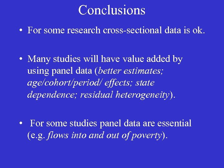Conclusions • For some research cross-sectional data is ok. • Many studies will have value added by using panel data (better estimates; age/cohort/period/ effects; state dependence; residual heterogeneity). • For some studies panel data are essential (e. g. flows into and out of poverty).

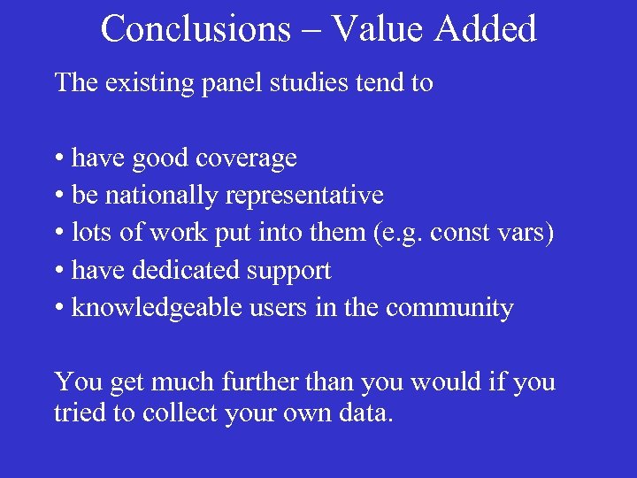Conclusions – Value Added The existing panel studies tend to • have good coverage • be nationally representative • lots of work put into them (e. g. const vars) • have dedicated support • knowledgeable users in the community You get much further than you would if you tried to collect your own data.

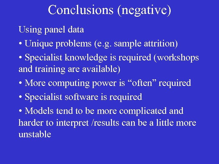Conclusions (negative) Using panel data • Unique problems (e. g. sample attrition) • Specialist knowledge is required (workshops and training are available) • More computing power is “often” required • Specialist software is required • Models tend to be more complicated and harder to interpret /results can be a little more unstable

OVERALL MESSAGE Panel data will usually add value to research projects. However, longitudinal data are not a panacea.