3734722bf22ec311f69f72baf319a8c1.ppt
- Количество слайдов: 33
 Long term exchange rates and inflation Purchasing power parity and the Balassa -Samuelson effect
: raised by 0. 25") Last Thursday • Fed increased its main rate (well expected): raised by 0. 25 the target range for the federal funds rate to 0. 75 per cent to 1 per cent • Market expectations for at least four Federal Reserve rate increases this year dipped to less than one-in-five
Last Thursday • Fed increased its main rate (well expected): raised by 0. 25 the target range for the federal funds rate to 0. 75 per cent to 1 per cent • Market expectations for at least four Federal Reserve rate increases this year dipped to less than one-in-five
 Motivation and roadmap • What are the determinants of exchange rates in the long term? • Why do poor countries have lower prices? Roadmap: • The law of one price, purchasing power parity (PPP): theory and empirics • The Balassa Samuelson effect: real exchange rates, growth and productivity
 • Long term perspective on exchange rates: when") The law of one price (LOP) • Long term perspective on exchange rates: when prices are flexible • On competitive markets, in absence of transport costs and tariffs…two identical goods must be sold at the same price (expressed in the same currency) • Pi € = E. Pi $ : long term arbitrage mechanism • If Pi € > E. Pi $ : buy the US produced good, sell it in Europe; increase demand in US, increase supply in Europe: price converge
The law of one price (LOP) • Long term perspective on exchange rates: when prices are flexible • On competitive markets, in absence of transport costs and tariffs…two identical goods must be sold at the same price (expressed in the same currency) • Pi € = E. Pi $ : long term arbitrage mechanism • If Pi € > E. Pi $ : buy the US produced good, sell it in Europe; increase demand in US, increase supply in Europe: price converge
 • P € = E. P $ where P €") Purchasing power parity (PPP) • P € = E. P $ where P € and P $ are price indices of US and euro zone • E = P € / P $ : Absolute version of PPP • Idea developed by Ricardo (1772– 1823 ) then Cassel (1866– 1945 ) • An increase in the general level of prices reduces purchasing power of domestic currency and leads to a depreciation • The price levels of different countries are equalized when measured in the same currency: P€ = E x P$
Purchasing power parity (PPP) • P € = E. P $ where P € and P $ are price indices of US and euro zone • E = P € / P $ : Absolute version of PPP • Idea developed by Ricardo (1772– 1823 ) then Cassel (1866– 1945 ) • An increase in the general level of prices reduces purchasing power of domestic currency and leads to a depreciation • The price levels of different countries are equalized when measured in the same currency: P€ = E x P$
 Relative PPP • The variation of the exchange rate is equal to the difference in the variation in prices, the difference in inflation rates (approximation) • Et = P €t / P $t ⇒ • (Et – Et-1)/Et-1 = π €t - π $t • π €t and π $t: inflation in € zone and US • π €t = (P€t – P€t-1)/ P€t-1
 • PPP in LT: E") The monetary approach to exchange rates (long term, LT) • PPP in LT: E = P € / P $ • Prices in LT: P€= MS€ / L (r€ , Y€) ; P$= MS$ / L (r$, Y$) where r€ , Y€ are LT values In LT, E is determined by relative supplies and demands of money in the two countries: E = P € / P $ = (MS€ / MS$ ) x [L (r$ , Y$)/L (r€ , Y€)] - MS€ ↑⇒ P € ↑ ⇒ € depreciation (how much depends on velocity of money, here =1) - Y€ ↑⇒ money demand ↑ ⇒ P € ↓ ⇒ € appreciation - r€ ↑ ⇒ money demand ↓⇒ P € ↑ ⇒ € depreciation
The monetary approach to exchange rates (long term, LT) • PPP in LT: E = P € / P $ • Prices in LT: P€= MS€ / L (r€ , Y€) ; P$= MS$ / L (r$, Y$) where r€ , Y€ are LT values In LT, E is determined by relative supplies and demands of money in the two countries: E = P € / P $ = (MS€ / MS$ ) x [L (r$ , Y$)/L (r€ , Y€)] - MS€ ↑⇒ P € ↑ ⇒ € depreciation (how much depends on velocity of money, here =1) - Y€ ↑⇒ money demand ↑ ⇒ P € ↓ ⇒ € appreciation - r€ ↑ ⇒ money demand ↓⇒ P € ↑ ⇒ € depreciation
 • In LT, interest parity condition is also verified: r€") The Fisher effect (1) • In LT, interest parity condition is also verified: r€ = r$ + (Ee – E)/ E • In LT: relative PPP (Et – Et-1)/Et-1 = π €t - π $t implies that expected depreciation equals expected inflation differential: • (Ee – E)/ E = πe€ - πe $ where • π e€ = (Pe€ – P €)/ P €
The Fisher effect (1) • In LT, interest parity condition is also verified: r€ = r$ + (Ee – E)/ E • In LT: relative PPP (Et – Et-1)/Et-1 = π €t - π $t implies that expected depreciation equals expected inflation differential: • (Ee – E)/ E = πe€ - πe $ where • π e€ = (Pe€ – P €)/ P €
 • So: r€ - r$ = (Ee – E)/ E") The Fisher effect (2) • So: r€ - r$ = (Ee – E)/ E = π e€ - πe $ • If expected inflation in euro zone is lower than in the US, the nominal interest rate r€ will also be lower • In LT, a higher nominal interest rate reflects expectations of higher inflation: this explains the association of high interest rate and depreciation in LT in the data • see today 10 year interest rates US = 2. 6% (2% 2 years ago); Germany: +0. 45% (0. 33% 2 years ago) • The ST and LT links between interest rates and exchange rate changes are opposite!
The Fisher effect (2) • So: r€ - r$ = (Ee – E)/ E = π e€ - πe $ • If expected inflation in euro zone is lower than in the US, the nominal interest rate r€ will also be lower • In LT, a higher nominal interest rate reflects expectations of higher inflation: this explains the association of high interest rate and depreciation in LT in the data • see today 10 year interest rates US = 2. 6% (2% 2 years ago); Germany: +0. 45% (0. 33% 2 years ago) • The ST and LT links between interest rates and exchange rate changes are opposite!
 Empirical validity of the LOP • LOP fails: not puzzling for non traded goods (haircuts) • More puzzling for traded goods
 The usual suspects behind the empirical failure of the LOP – Transport costs, trade barriers (tariffs and regulations): make arbitrage more difficult – On purpose: lobbies to regulate markets differently to weaken competition – Imperfect competition: firms want to segment markets (to have high prices where price elasticity of demand is low) : “pricing to market” – Many goods considered to be highly traded contain nontraded components. Retail and wholesale costs (distribution costs) account for around 50% of final consumer price
 Price differences for a selection of best-selling cars (% of prices in euro before tax, comparing the most expensive with the cheapest euro zone market)
 Berka, Devereux, Engel, 2014, Real Exchange Rates and Sectoral Productivity in the Eurozone; NBER Working Paper No. 20510
 Price dispersion across and within Eurozone countries
 Empirical validity of PPP • Studies overwhelmingly reject PPP as a short -run relationship, better as long term • The failure of short-run PPP can be attributed mostly to the stickiness in nominal prices (short run) • In long term (after 4 -5 years) evidence that exchange rates converge to PPP levels
 The Yen/$ exchange rate and the relative price ratio over the long term
 defined as the relative") Long term real exchange rate • Real exchange rate (RER) defined as the relative price index of goods and services between two countries: q = E x P $ / P € (can also be computed inside € zone) A real depreciation of € vis a vis the $ (q ) can come from nominal depreciation (E ), an increase in P $ or a fall in P € • Relative PPP ⇒ RER is constant • PPP: (Et – Et-1)/Et-1 = π €t - π $t • (qt – qt-1)/qt-1 = (Et – Et-1)/Et-1 - π €t + π $t = 0
Long term real exchange rate • Real exchange rate (RER) defined as the relative price index of goods and services between two countries: q = E x P $ / P € (can also be computed inside € zone) A real depreciation of € vis a vis the $ (q ) can come from nominal depreciation (E ), an increase in P $ or a fall in P € • Relative PPP ⇒ RER is constant • PPP: (Et – Et-1)/Et-1 = π €t - π $t • (qt – qt-1)/qt-1 = (Et – Et-1)/Et-1 - π €t + π $t = 0
 The Balassa-Samuelson effect • Why are prices higher in rich countries? • Same question as: why E x P rich > P poor? • Why does the real exchange rate of countries that grow relative to rest of world appreciate? q = E x Pworld / P ↓ • Examples: Japan, South Korea, Ireland, today China?
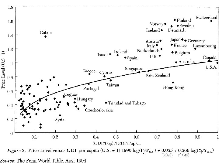
 and non tradable (services)") Balassa Samuelson model: • Key distinction: Tradable goods (manufactured goods) and non tradable (services) • Around 75% of the consumption basket in industrialized countries is non tradable (health, education, most services…) • Productivity differences between rich and poor countries much larger for tradables than for non tradables: very large in manufacturing (around 10 between average industrialized and debelopping country), but much smaller in services (haircuts: technology not so different across countries)
Balassa Samuelson model: • Key distinction: Tradable goods (manufactured goods) and non tradable (services) • Around 75% of the consumption basket in industrialized countries is non tradable (health, education, most services…) • Productivity differences between rich and poor countries much larger for tradables than for non tradables: very large in manufacturing (around 10 between average industrialized and debelopping country), but much smaller in services (haircuts: technology not so different across countries)
 Price index (CPI) depends on") • 2 countries: Poor country, rich country (*) Price index (CPI) depends on tradables (T) and non tradables • P = (PT)a x (PN)1 -a ; P* = (P*T)a x (P*N)1 -a • Share a and 1 -a (around 25% and 75%) • One factor of production: labor • Mobile between sectors (in long term) but not between countries • Identical countries except in productivity
• 2 countries: Poor country, rich country (*) Price index (CPI) depends on tradables (T) and non tradables • P = (PT)a x (PN)1 -a ; P* = (P*T)a x (P*N)1 -a • Share a and 1 -a (around 25% and 75%) • One factor of production: labor • Mobile between sectors (in long term) but not between countries • Identical countries except in productivity
 • Labor is mobile between sectors in LT: Arbitrage ⇒ w = w. T = w. N ; w*= w*T = w*N Profit max. by firms ⇒ marginal cost of labor = marginal value of employing one more unit of labor: for example in T: w = PT AT AT: marginal productivity of labor (nb of units of goods produced with one more unit of labor) real wage = marginal productivity of labor : w / PT = A T ; w/ PN = AN w* / P*T = A*T ; w* / P*N = A*N
 Choose numeraire so that E =") PPP for tradable goods (not for non tradables) Choose numeraire so that E = 1 (normalization with no real consequence): PT = P*T and PT = w / AT P*T = w* / A*T →w / AT = w*/A*T so w/w* = AT / A*T First result: wages in poorer countries are lower because of lower productivity in tradables Wages in non tradables also lower in poorer countries: wages are equalized by arbitrage across sectors inside each country
PPP for tradable goods (not for non tradables) Choose numeraire so that E = 1 (normalization with no real consequence): PT = P*T and PT = w / AT P*T = w* / A*T →w / AT = w*/A*T so w/w* = AT / A*T First result: wages in poorer countries are lower because of lower productivity in tradables Wages in non tradables also lower in poorer countries: wages are equalized by arbitrage across sectors inside each country
/ (w* /A*N) = (AT /") Balassa Samuelson effect PN / P*N = (w /AN)/ (w* /A*N) = (AT / A*T)/(AN / A*N) as PN = w /AN , P*N = w/ A*N and w/w* = AT / A*T The relative price of non tradables depends on the relative productivities in the tradable and non tradable sectors
Balassa Samuelson effect PN / P*N = (w /AN)/ (w* /A*N) = (AT / A*T)/(AN / A*N) as PN = w /AN , P*N = w/ A*N and w/w* = AT / A*T The relative price of non tradables depends on the relative productivities in the tradable and non tradable sectors
: (PT)a x (PN)1 -a =") Relative Price index between countries (use PPP on tradables): (PT)a x (PN)1 -a = P/P* = (P*T)a x (P*N)1 -a (Use PPP in T PT = P*T) (P*N)1 -a
Relative Price index between countries (use PPP on tradables): (PT)a x (PN)1 -a = P/P* = (P*T)a x (P*N)1 -a (Use PPP in T PT = P*T) (P*N)1 -a
 Balassa Samuelson effect Relative prices between countries depends on relative productivities between tradables and non tradables: (AT / A*T)1 -a P/P* = < 1 if AT / A*T < AN / A*N (AN / A*N)1 -a The productivity differential between poor and rich countries much larger in T (AT << A*T) than in N (AN < A*N) No effect on relative prices P/P* if international productivity gap equal in both sectors
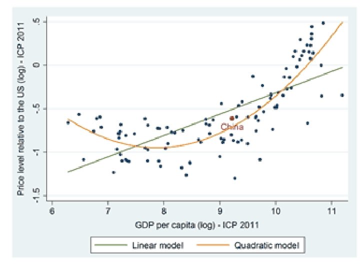
 Balassa Samuelson effect Poorer countries have lower wages in tradables because of lower productivity in tradables; these translate in lower wages in non tradables and lower non tradables prices (productivity gap not as large in NT) lower prices in poorer countries As a country gets richer, AT increases (more than AN ); wages in the T sector ↑ and therefore in the N sector too. Its price index increases relative to other countries China? How does its RER compare to what is predicted by Balassa Samuelson? ln(RER) = constant + a ln (GDP/capita)
 China’s real effective exchange rate: q = EP*/P Where E, P* are weighted exchange rate and foreign prices (weighted by trade share with China) q decreases means real apppreciation 130 120 110 100 REER 90 NEER 80 70 01 1 -2 01 01 2 -2 01 01 3 -2 01 01 4 -2 01 01 5 -2 01 01 6 -2 01 7 01 -2 01 0 01 -2 00 9 01 -2 08 01 20 00 7 01 - -2 00 6 01 -2 00 5 01 -2 00 4 01 -2 00 3 01 -2 00 2 01 -2 00 1 01 -2 00 0 60 Source: BIS, 2010=100
 China real exchange rate expected to appreciate • Real effective appreciation of around 20% since 2010 (mostly through nominal appreciation): expected from fast growing country (Balassa Samuelson) • China is still a relatively poor country (GDP/cap): lower prices than in OECD countries (PPP should not hold for CPIs: Yuan may not be so undervalued) • But as converges to GDP/cap of OECD will appreciate (nominal appreciation or inflation)
. Careful here up") In 2000 , 36% undervalued (with respect to Balassa Samuelson prediction). Careful here up is appreciation (just to confuse you…) The Balassa-Samuelson Relationship and the Renminbi, Jeffrey Frankel, december 2006
In 2000 , 36% undervalued (with respect to Balassa Samuelson prediction). Careful here up is appreciation (just to confuse you…) The Balassa-Samuelson Relationship and the Renminbi, Jeffrey Frankel, december 2006