91ddaef1c419d4510f0534e698f59bba.ppt
- Количество слайдов: 66
Logit/Probit Models 1
Making sense of the decision rule • Suppose we have a kid with great scores, great grades, etc. • For this kid, xi β is large. • What will prevent admission? Only a large negative εi • What is the probability of observing a large negative εi ? Very small. • Most likely admitted. We estimate a large probability 2
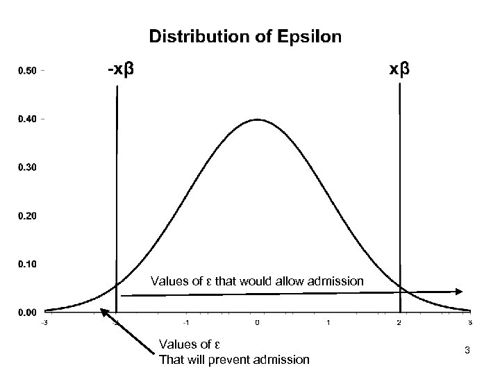
Values of ε that would allow admission Values of ε That will prevent admission 3
Another example • Suppose we have a kid with bad scores. • For this kid, xi β is small (even negative). • What will allow admission? Only a large positive εi • What is the probability of observing a large positive εi ? Very small. • Most likely, not admitted, so, we estimate a small probability 4
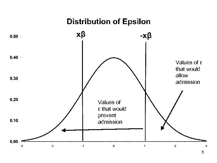
Values of ε that would allow admission Values of ε that would prevent admission 5
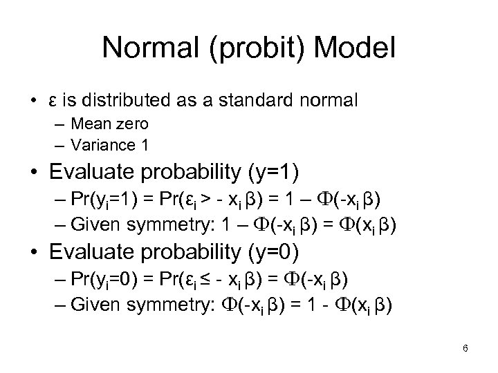
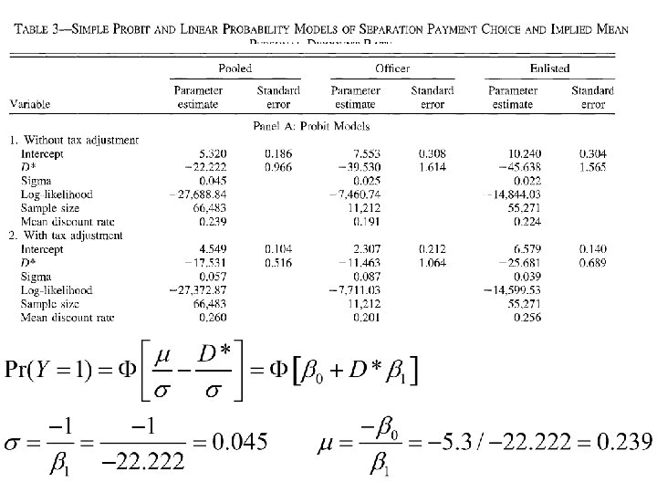
Normal (probit) Model • ε is distributed as a standard normal – Mean zero – Variance 1 • Evaluate probability (y=1) – Pr(yi=1) = Pr(εi > - xi β) = 1 – Ф(-xi β) – Given symmetry: 1 – Ф(-xi β) = Ф(xi β) • Evaluate probability (y=0) – Pr(yi=0) = Pr(εi ≤ - xi β) = Ф(-xi β) – Given symmetry: Ф(-xi β) = 1 - Ф(xi β) 6
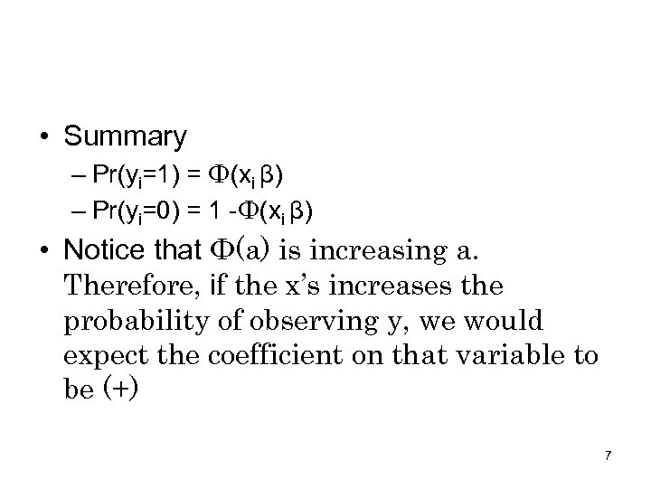
• Summary – Pr(yi=1) = Ф(xi β) – Pr(yi=0) = 1 -Ф(xi β) • Notice that Ф(a) is increasing a. Therefore, if the x’s increases the probability of observing y, we would expect the coefficient on that variable to be (+) 7
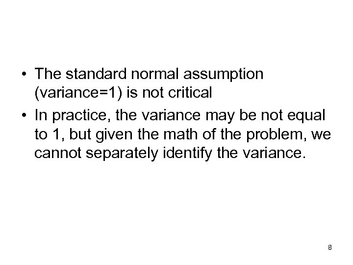
• The standard normal assumption (variance=1) is not critical • In practice, the variance may be not equal to 1, but given the math of the problem, we cannot separately identify the variance. 8
![Logit • PDF: f(x) = exp(x)/[1+exp(x)]2 • CDF: F(a) = exp(a)/[1+exp(a)] – Symmetric, unimodal Logit • PDF: f(x) = exp(x)/[1+exp(x)]2 • CDF: F(a) = exp(a)/[1+exp(a)] – Symmetric, unimodal](https://present5.com/presentation/91ddaef1c419d4510f0534e698f59bba/image-9.jpg)
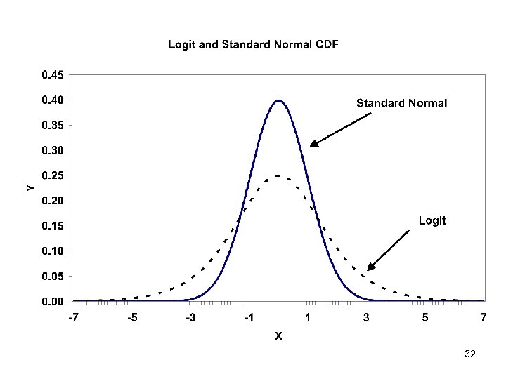
Logit • PDF: f(x) = exp(x)/[1+exp(x)]2 • CDF: F(a) = exp(a)/[1+exp(a)] – Symmetric, unimodal distribution – Looks a lot like the normal – Incredibly easy to evaluate the CDF and PDF – Mean of zero, variance > 1 (more variance than normal) 9
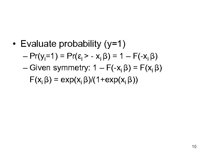
• Evaluate probability (y=1) – Pr(yi=1) = Pr(εi > - xi β) = 1 – F(-xi β) – Given symmetry: 1 – F(-xi β) = F(xi β) = exp(xi β)/(1+exp(xi β)) 10
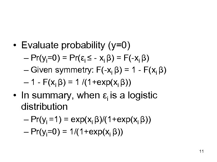
• Evaluate probability (y=0) – Pr(yi=0) = Pr(εi ≤ - xi β) = F(-xi β) – Given symmetry: F(-xi β) = 1 - F(xi β) – 1 - F(xi β) = 1 /(1+exp(xi β)) • In summary, when εi is a logistic distribution – Pr(yi =1) = exp(xi β)/(1+exp(xi β)) – Pr(yi=0) = 1/(1+exp(xi β)) 11
STATA Resources Discrete Outcomes • “Regression Models for Categorical Dependent Variables Using STATA” – J. Scott Long and Jeremy Freese • Available for sale from STATA website for $52 (www. stata. com) • Post-estimation subroutines that translate results – Do not need to buy the book to use the subroutines 12

• In STATA command line type • net search spost • Will give you a list of available programs to download • One is Spostado from http: //www. indiana. edu/~jslsoc/stata • Click on the link and install the files 13
Example: Workplace smoking bans • Smoking supplements to 1991 and 1993 National Health Interview Survey • Asked all respondents whether they currently smoke • Asked workers about workplace tobacco policies • Sample: indoor workers • Key variables: current smoking and whether they faced a workplace ban 14

• Data: workplace 1. dta • Sample program: workplace 1. doc • Results: workplace 1. log 15
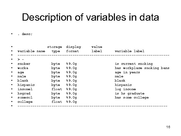
Description of variables in data • . desc; • • • • storage display value variable name type format label variable label ------------------------------------> smoker byte %9. 0 g is current smoking worka byte %9. 0 g has workplace smoking bans age byte %9. 0 g age in years male byte %9. 0 g male black byte %9. 0 g black hispanic byte %9. 0 g hispanic incomel float %9. 0 g log income hsgrad byte %9. 0 g is hs graduate somecol byte %9. 0 g has some college float %9. 0 g ------------------------------------ 16
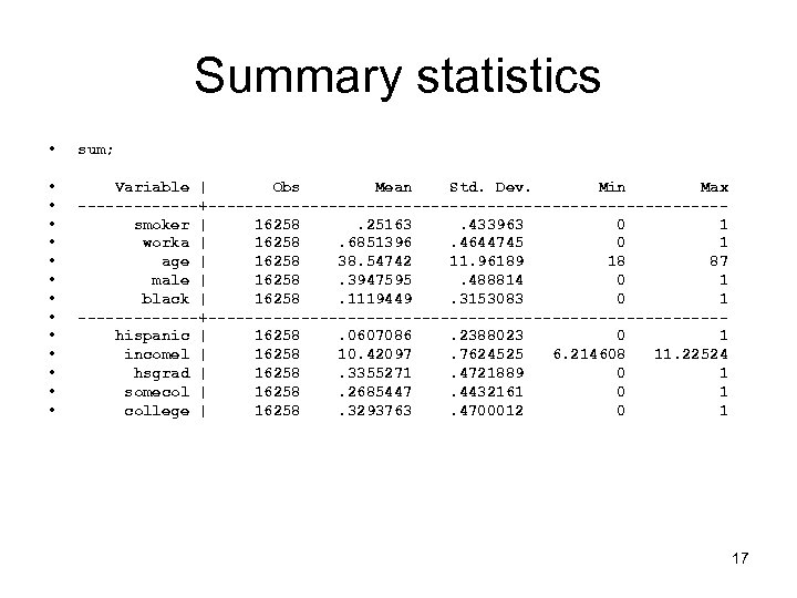
Summary statistics • sum; • • • • Variable | Obs Mean Std. Dev. Min Max -------+----------------------------smoker | 16258. 25163. 433963 0 1 worka | 16258. 6851396. 4644745 0 1 age | 16258 38. 54742 11. 96189 18 87 male | 16258. 3947595. 488814 0 1 black | 16258. 1119449. 3153083 0 1 -------+----------------------------hispanic | 16258. 0607086. 2388023 0 1 incomel | 16258 10. 42097. 7624525 6. 214608 11. 22524 hsgrad | 16258. 3355271. 4721889 0 1 somecol | 16258. 2685447. 4432161 0 1 college | 16258. 3293763. 4700012 0 1 17
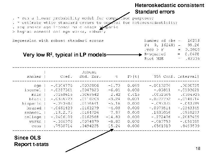
Heteroskedastic consistent Standard errors Very low R 2, typical in LP models Since OLS Report t-stats 18
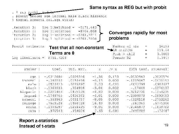
Same syntax as REG but with probit Converges rapidly for most problems Test that all non-constant Terms are 0 Report z-statistics Instead of t-stats 19
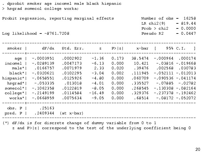
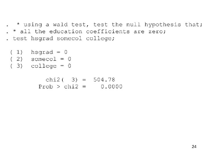
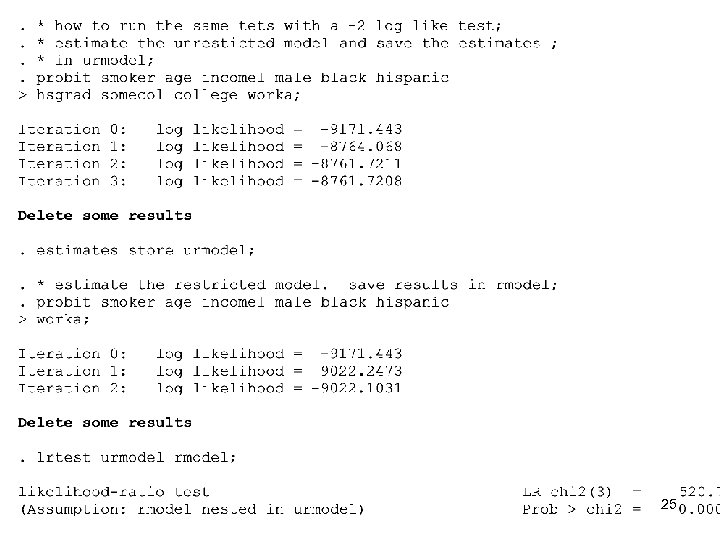
. dprobit smoker age incomel male black hispanic > hsgrad somecol college worka; Probit regression, reporting marginal effects Log likelihood = -8761. 7208 Number of obs LR chi 2(9) Prob > chi 2 Pseudo R 2 = 16258 = 819. 44 = 0. 0000 = 0. 0447 ---------------------------------------smoker | d. F/dx Std. Err. z P>|z| x-bar [ 95% C. I. ] -----+----------------------------------age | -. 0003951. 0002902 -1. 36 0. 173 38. 5474 -. 000964. 000174 incomel | -. 0289139. 0047173 -6. 13 0. 000 10. 421 -. 03816 -. 019668 male*|. 0166757. 0071979 2. 33 0. 020. 39476. 002568. 030783 black*| -. 0320621. 0102295 -3. 04 0. 002. 111945 -. 052111 -. 012013 hispanic*| -. 0658551. 0125926 -4. 80 0. 000. 060709 -. 090536 -. 041174 hsgrad*| -. 053335. 013018 -4. 01 0. 000. 335527 -. 07885 -. 02782 somecol*| -. 1062358. 0122819 -8. 05 0. 000. 268545 -. 130308 -. 082164 college*| -. 2149199. 0114584 -16. 49 0. 000. 329376 -. 237378 -. 192462 worka*| -. 0668959. 0075634 -9. 05 0. 000. 68514 -. 08172 -. 052072 -----+----------------------------------obs. P |. 25163 pred. P |. 2409344 (at x-bar) ---------------------------------------(*) d. F/dx is for discrete change of dummy variable from 0 to 1 z and P>|z| correspond to the test of the underlying coefficient being 0 20
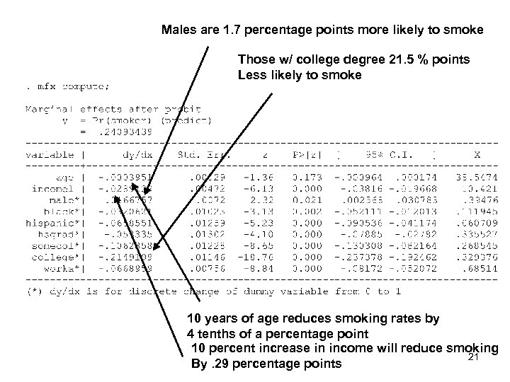
Males are 1. 7 percentage points more likely to smoke Those w/ college degree 21. 5 % points Less likely to smoke 10 years of age reduces smoking rates by 4 tenths of a percentage point 10 percent increase in income will reduce smoking 21 By. 29 percentage points
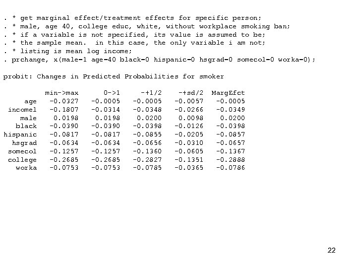
. . . * get marginal effect/treatment effects for specific person; * male, age 40, college educ, white, without workplace smoking ban; * if a variable is not specified, its value is assumed to be; * the sample mean. in this case, the only variable i am not; * listing is mean log income; prchange, x(male=1 age=40 black=0 hispanic=0 hsgrad=0 somecol=0 worka=0); probit: Changes in Predicted Probabilities for smoker age incomel male black hispanic hsgrad somecol college worka min->max -0. 0327 -0. 1807 0. 0198 -0. 0390 -0. 0817 -0. 0634 -0. 1257 -0. 2685 -0. 0753 0 ->1 -0. 0005 -0. 0314 0. 0198 -0. 0390 -0. 0817 -0. 0634 -0. 1257 -0. 2685 -0. 0753 -+1/2 -0. 0005 -0. 0348 0. 0200 -0. 0398 -0. 0855 -0. 0656 -0. 1360 -0. 2827 -0. 0785 -+sd/2 -0. 0057 -0. 0266 0. 0098 -0. 0126 -0. 0205 -0. 0310 -0. 0605 -0. 1351 -0. 0365 Marg. Efct -0. 0005 -0. 0349 0. 0200 -0. 0398 -0. 0857 -0. 0657 -0. 1367 -0. 2888 -0. 0786 22
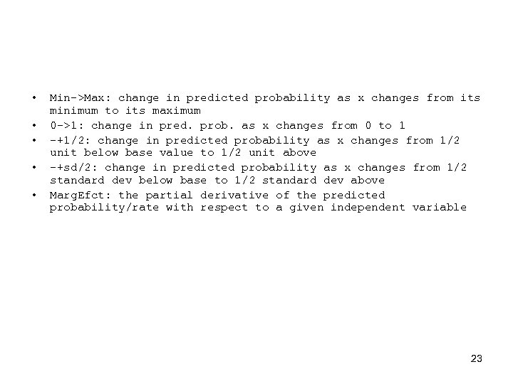
• • • Min->Max: change in predicted probability as x changes from its minimum to its maximum 0 ->1: change in pred. prob. as x changes from 0 to 1 -+1/2: change in predicted probability as x changes from 1/2 unit below base value to 1/2 unit above -+sd/2: change in predicted probability as x changes from 1/2 standard dev below base to 1/2 standard dev above Marg. Efct: the partial derivative of the predicted probability/rate with respect to a given independent variable 23
24
25
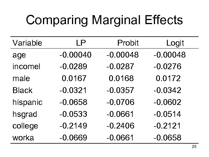
Comparing Marginal Effects Variable age incomel male Black hispanic hsgrad college worka LP -0. 00040 -0. 0289 0. 0167 -0. 0321 -0. 0658 -0. 0533 -0. 2149 -0. 0669 Probit -0. 00048 -0. 0287 0. 0168 -0. 0357 -0. 0706 -0. 0661 -0. 2406 -0. 0661 Logit -0. 00048 -0. 0276 0. 0172 -0. 0342 -0. 0602 -0. 0514 -0. 2121 -0. 0658 26
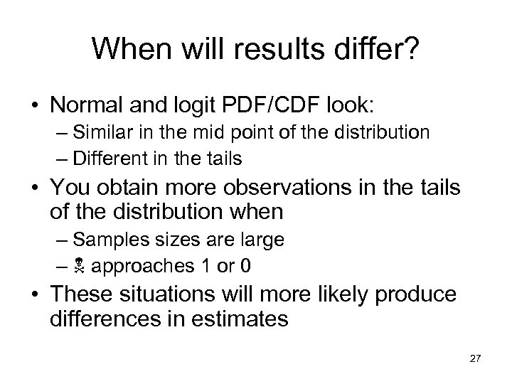
When will results differ? • Normal and logit PDF/CDF look: – Similar in the mid point of the distribution – Different in the tails • You obtain more observations in the tails of the distribution when – Samples sizes are large – approaches 1 or 0 • These situations will more likely produce differences in estimates 27
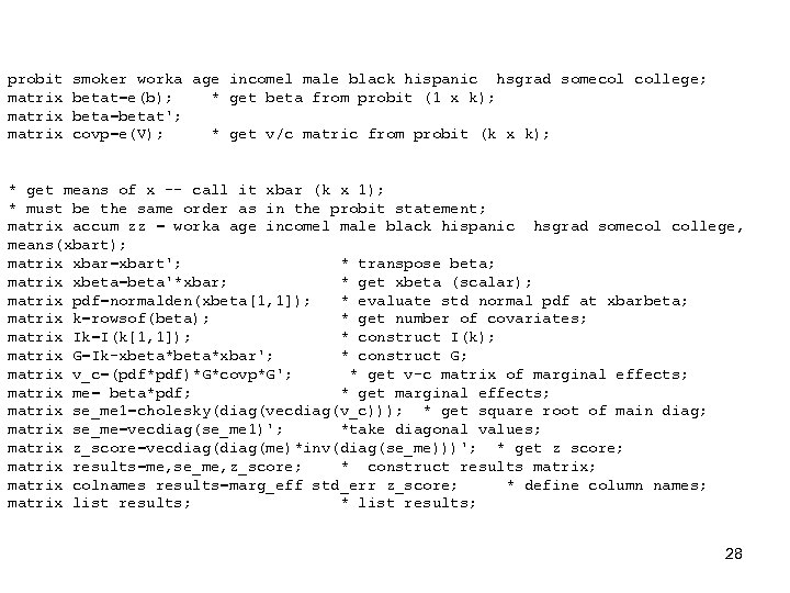
probit matrix smoker worka age incomel male black hispanic hsgrad somecol college; betat=e(b); * get beta from probit (1 x k); beta=betat'; covp=e(V); * get v/c matric from probit (k x k); * get means of x -- call it xbar (k x 1); * must be the same order as in the probit statement; matrix accum zz = worka age incomel male black hispanic hsgrad somecol college, means(xbart); matrix xbar=xbart'; * transpose beta; matrix xbeta=beta'*xbar; * get xbeta (scalar); matrix pdf=normalden(xbeta[1, 1]); * evaluate std normal pdf at xbarbeta; matrix k=rowsof(beta); * get number of covariates; matrix Ik=I(k[1, 1]); * construct I(k); matrix G=Ik-xbeta*xbar'; * construct G; matrix v_c=(pdf*pdf)*G*covp*G'; * get v-c matrix of marginal effects; matrix me= beta*pdf; * get marginal effects; matrix se_me 1=cholesky(diag(vecdiag(v_c))); * get square root of main diag; matrix se_me=vecdiag(se_me 1)'; *take diagonal values; matrix z_score=vecdiag(me)*inv(diag(se_me)))'; * get z score; matrix results=me, se_me, z_score; * construct results matrix; matrix colnames results=marg_eff std_err z_score; * define column names; matrix list results; * list results; 28
![results[10, 3] marg_eff worka -. 06521255 age -. 00039515 incomel -. 02891389 male. 01661127 results[10, 3] marg_eff worka -. 06521255 age -. 00039515 incomel -. 02891389 male. 01661127](https://present5.com/presentation/91ddaef1c419d4510f0534e698f59bba/image-29.jpg)
results[10, 3] marg_eff worka -. 06521255 age -. 00039515 incomel -. 02891389 male. 01661127 black -. 03303852 hispanic -. 07107496 hsgrad -. 05447959 somecol -. 11335675 college -. 23955322 _cons. 2712018 std_err. 00720374. 00029023. 00471728. 00714305. 0108782. 01479806. 01359844. 01408096. 0144803. 04808183 z_score -9. 0525984 -1. 3615156 -6. 129356 2. 3255154 -3. 0371321 -4. 8029926 -4. 0063111 -8. 0503576 -16. 543383 5. 6404217 ---------------------------------------smoker | d. F/dx Std. Err. z P>|z| x-bar [ 95% C. I. ] -----+----------------------------------age | -. 0003951. 0002902 -1. 36 0. 173 38. 5474 -. 000964. 000174 incomel | -. 0289139. 0047173 -6. 13 0. 000 10. 421 -. 03816 -. 019668 male*|. 0166757. 0071979 2. 33 0. 020. 39476. 002568. 030783 black*| -. 0320621. 0102295 -3. 04 0. 002. 111945 -. 052111 -. 012013 hispanic*| -. 0658551. 0125926 -4. 80 0. 000. 060709 -. 090536 -. 041174 hsgrad*| -. 053335. 013018 -4. 01 0. 000. 335527 -. 07885 -. 02782 somecol*| -. 1062358. 0122819 -8. 05 0. 000. 268545 -. 130308 -. 082164 college*| -. 2149199. 0114584 -16. 49 0. 000. 329376 -. 237378 -. 192462 worka*| -. 0668959. 0075634 -9. 05 0. 000. 68514 -. 08172 -. 052072 -----+----------------------------------29

* this is an example of a marginal effect for a dichotomous outcome; * in this case, set the 1 st variable worka as 1 or 0; matrix x 1=xbar; matrix x 1[1, 1]=1; matrix x 0=xbar; matrix x 0[1, 1]=0; matrix xbeta 1=beta'*x 1; matrix xbeta 0=beta'*x 0; matrix prob 1=normal(xbeta 1[1, 1]); matrix prob 0=normal(xbeta 0[1, 1]); matrix me_1=prob 1 -prob 0; matrix pdf 1=normalden(xbeta 1[1, 1]); matrix pdf 0=normalden(xbeta 0[1, 1]); matrix G 1=pdf 1*x 1 - pdf 0*x 0; matrix v_c 1=G 1'*covp*G 1; matrix se_me_1=sqrt(v_c 1[1, 1]); * marginal effect of workplace bans; matrix list me_1; * standard error of workplace a; matrix list se_me_1; 30
![symmetric me_1[1, 1] c 1 r 1 -. 06689591. * standard error of workplace symmetric me_1[1, 1] c 1 r 1 -. 06689591. * standard error of workplace](https://present5.com/presentation/91ddaef1c419d4510f0534e698f59bba/image-31.jpg)
symmetric me_1[1, 1] c 1 r 1 -. 06689591. * standard error of workplace a; . matrix list se_me_1; symmetric se_me_1[1, 1] c 1 r 1. 00756336 ---------------------------------------smoker | d. F/dx Std. Err. z P>|z| x-bar [ 95% C. I. ] -----+----------------------------------age | -. 0003951. 0002902 -1. 36 0. 173 38. 5474 -. 000964. 000174 incomel | -. 0289139. 0047173 -6. 13 0. 000 10. 421 -. 03816 -. 019668 male*|. 0166757. 0071979 2. 33 0. 020. 39476. 002568. 030783 black*| -. 0320621. 0102295 -3. 04 0. 002. 111945 -. 052111 -. 012013 hispanic*| -. 0658551. 0125926 -4. 80 0. 000. 060709 -. 090536 -. 041174 hsgrad*| -. 053335. 013018 -4. 01 0. 000. 335527 -. 07885 -. 02782 somecol*| -. 1062358. 0122819 -8. 05 0. 000. 268545 -. 130308 -. 082164 college*| -. 2149199. 0114584 -16. 49 0. 000. 329376 -. 237378 -. 192462 worka*| -. 0668959. 0075634 -9. 05 0. 000. 68514 -. 08172 -. 052072 -----+----------------------------------31
32
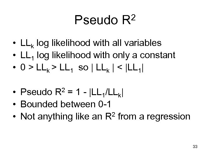
Pseudo R 2 • LLk log likelihood with all variables • LL 1 log likelihood with only a constant • 0 > LLk > LL 1 so | LLk | < |LL 1| • Pseudo R 2 = 1 - |LL 1/LLk| • Bounded between 0 -1 • Not anything like an R 2 from a regression 33
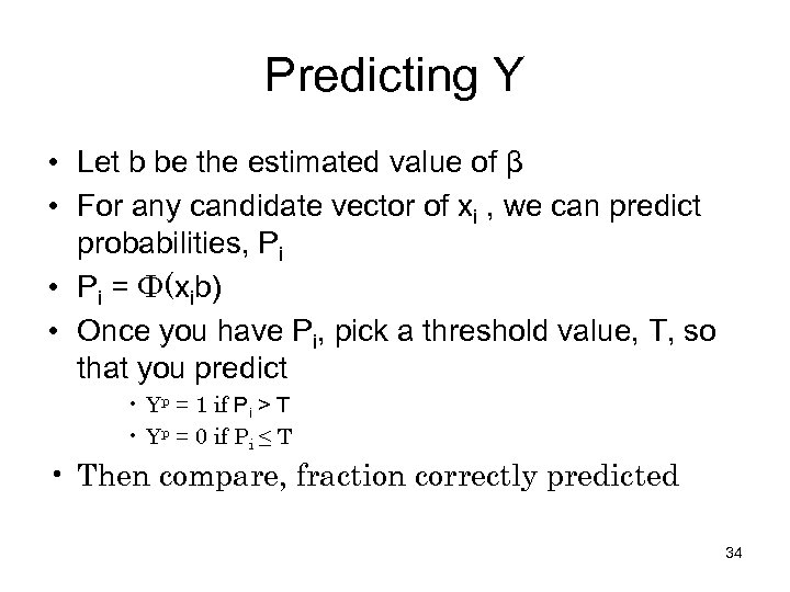
Predicting Y • Let b be the estimated value of β • For any candidate vector of xi , we can predict probabilities, Pi • Pi = Ф(xib) • Once you have Pi, pick a threshold value, T, so that you predict • Yp = 1 if Pi > T • Yp = 0 if Pi ≤ T • Then compare, fraction correctly predicted 34
• Question: what value to pick for T? • Can pick. 5 – what some textbooks suggest – Intuitive. More likely to engage in the activity than to not engage in it – When is small (large), this criteria does a poor job of predicting Yi=1 (Yi=0) 35
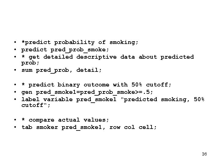
• *predict probability of smoking; • predict pred_prob_smoke; • * get detailed descriptive data about predicted prob; • sum pred_prob, detail; • * predict binary outcome with 50% cutoff; • gen pred_smoke 1=pred_prob_smoke>=. 5; • label variable pred_smoke 1 "predicted smoking, 50% cutoff"; • * compare actual values; • tab smoker pred_smoke 1, row col cell; 36
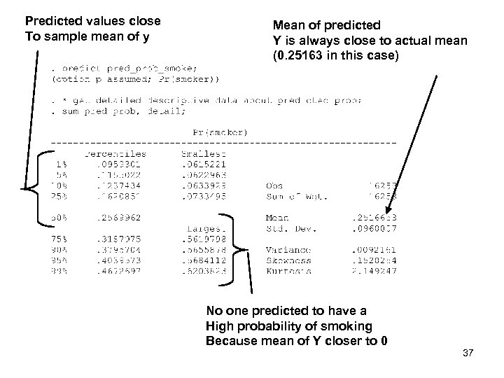
Predicted values close To sample mean of y Mean of predicted Y is always close to actual mean (0. 25163 in this case) No one predicted to have a High probability of smoking Because mean of Y closer to 0 37
Some nice properties of the Logit • Outcome, y=1 or 0 • Treatment, x=1 or 0 • Other covariates, x • Context, – x = whether a baby is born with a low weight birth – x = whether the mom smoked or not during pregnancy 38
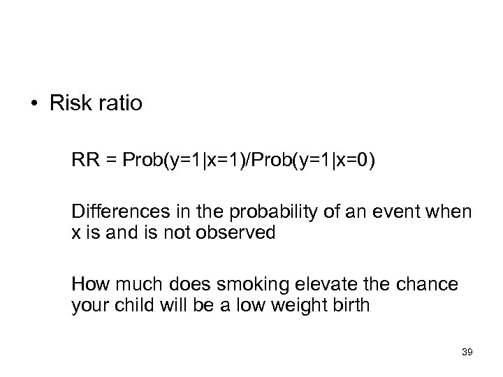
• Risk ratio RR = Prob(y=1|x=1)/Prob(y=1|x=0) Differences in the probability of an event when x is and is not observed How much does smoking elevate the chance your child will be a low weight birth 39
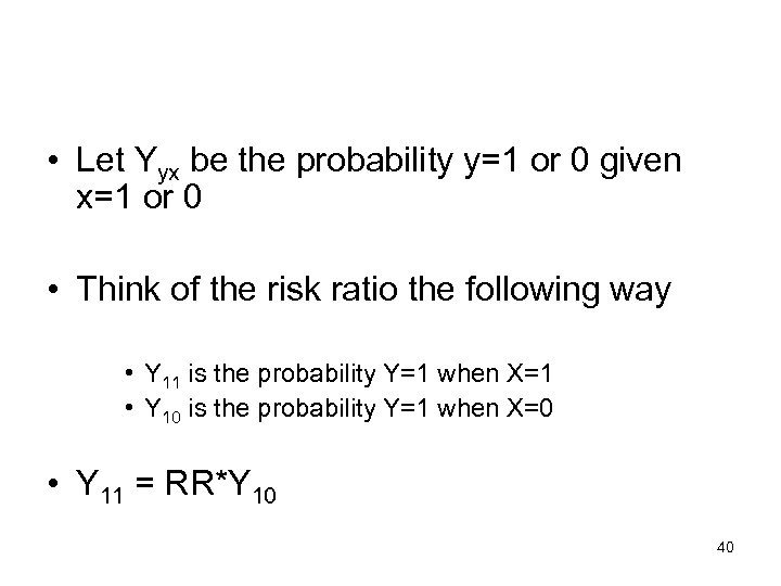
• Let Yyx be the probability y=1 or 0 given x=1 or 0 • Think of the risk ratio the following way • Y 11 is the probability Y=1 when X=1 • Y 10 is the probability Y=1 when X=0 • Y 11 = RR*Y 10 40
![• Odds Ratio OR=A/B = [Y 11/Y 01]/[Y 10/Y 00] A = [Pr(Y=1|X=1)/Pr(Y=0|X=1)] • Odds Ratio OR=A/B = [Y 11/Y 01]/[Y 10/Y 00] A = [Pr(Y=1|X=1)/Pr(Y=0|X=1)]](https://present5.com/presentation/91ddaef1c419d4510f0534e698f59bba/image-41.jpg)
• Odds Ratio OR=A/B = [Y 11/Y 01]/[Y 10/Y 00] A = [Pr(Y=1|X=1)/Pr(Y=0|X=1)] = odds of Y occurring if you are a smoker B = [Pr(Y=1|X=0)/Pr(Y=0|X=0)] = odds of Y happening if you are not a smoker What are the relative odds of Y happening if you do or do not experience X 41
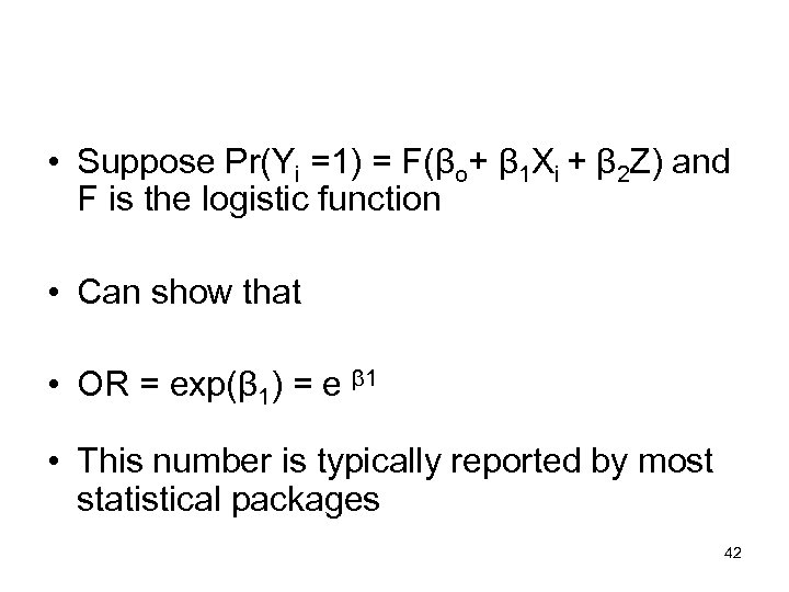
• Suppose Pr(Yi =1) = F(βo+ β 1 Xi + β 2 Z) and F is the logistic function • Can show that • OR = exp(β 1) = e β 1 • This number is typically reported by most statistical packages 42
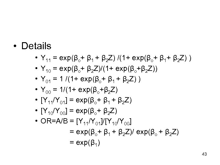
• Details • • Y 11 = exp(βo+ β 1 + β 2 Z) /(1+ exp(βo+ β 1+ β 2 Z) ) Y 10 = exp(βo+ β 2 Z)/(1+ exp(βo+β 2 Z)) Y 01 = 1 /(1+ exp(βo+ β 1 + β 2 Z) ) Y 00 = 1/(1+ exp(βo+β 2 Z) [Y 11/Y 01] = exp(βo+ β 1 + β 2 Z) [Y 10/Y 00] = exp(βo+ β 2 Z) OR=A/B = [Y 11/Y 01]/[Y 10/Y 00] = exp(βo+ β 1 + β 2 Z)/ exp(βo + β 2 Z) = exp(β 1) 43
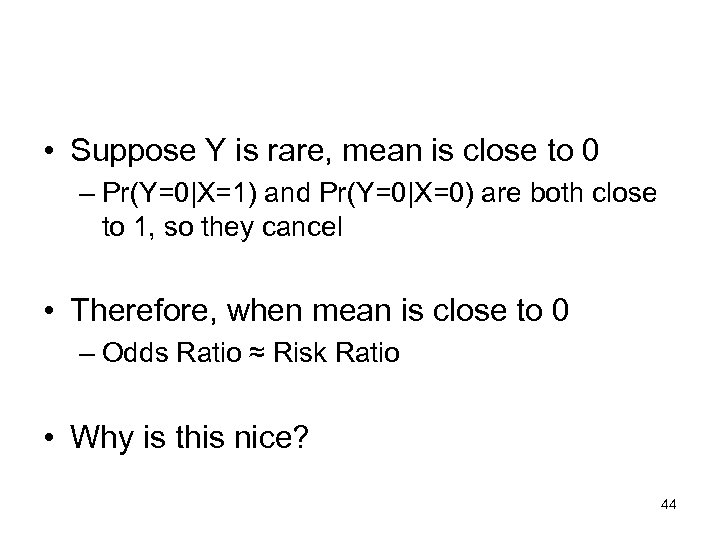
• Suppose Y is rare, mean is close to 0 – Pr(Y=0|X=1) and Pr(Y=0|X=0) are both close to 1, so they cancel • Therefore, when mean is close to 0 – Odds Ratio ≈ Risk Ratio • Why is this nice? 44
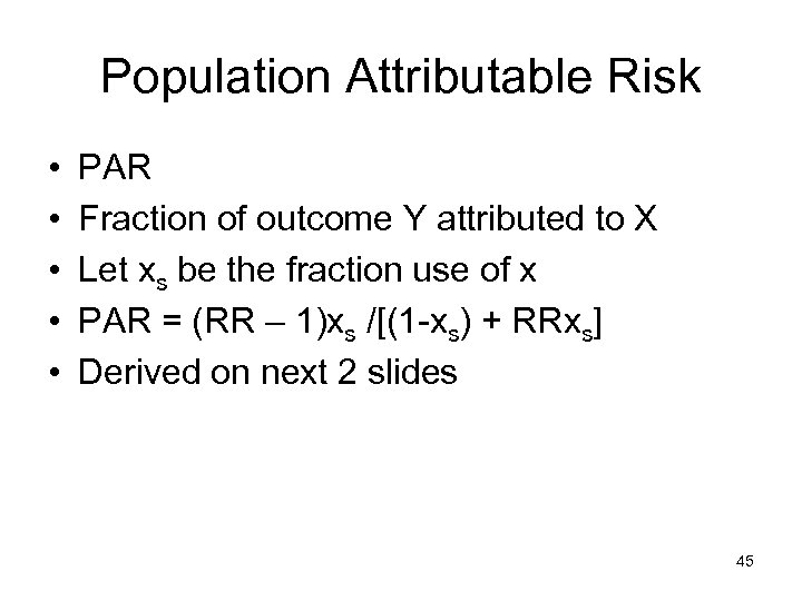
Population Attributable Risk • • • PAR Fraction of outcome Y attributed to X Let xs be the fraction use of x PAR = (RR – 1)xs /[(1 -xs) + RRxs] Derived on next 2 slides 45
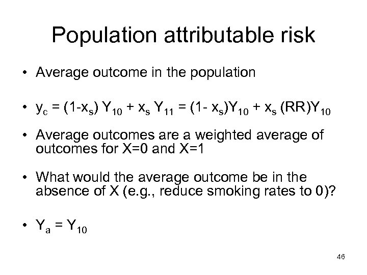
Population attributable risk • Average outcome in the population • yc = (1 -xs) Y 10 + xs Y 11 = (1 - xs)Y 10 + xs (RR)Y 10 • Average outcomes are a weighted average of outcomes for X=0 and X=1 • What would the average outcome be in the absence of X (e. g. , reduce smoking rates to 0)? • Ya = Y 10 46
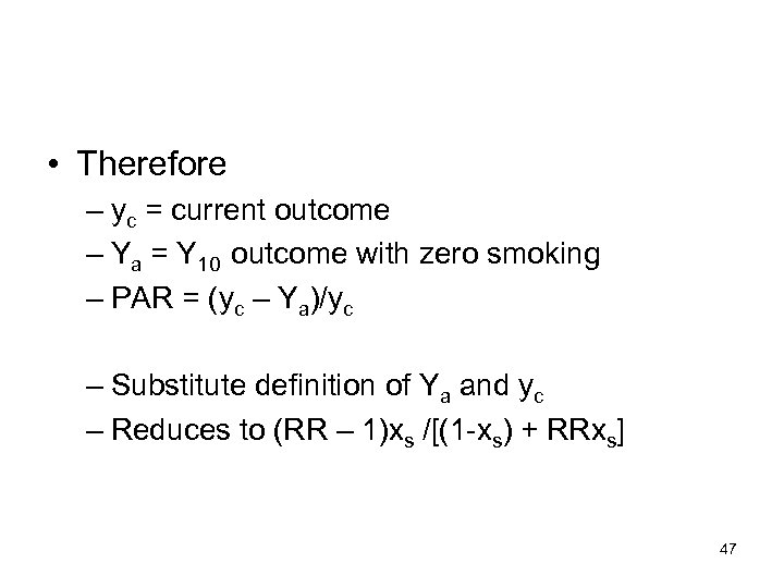
• Therefore – yc = current outcome – Ya = Y 10 outcome with zero smoking – PAR = (yc – Ya)/yc – Substitute definition of Ya and yc – Reduces to (RR – 1)xs /[(1 -xs) + RRxs] 47
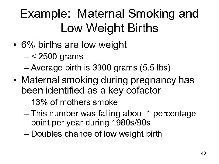
Example: Maternal Smoking and Low Weight Births • 6% births are low weight – < 2500 grams – Average birth is 3300 grams (5. 5 lbs) • Maternal smoking during pregnancy has been identified as a key cofactor – 13% of mothers smoke – This number was falling about 1 percentage point per year during 1980 s/90 s – Doubles chance of low weight birth 48
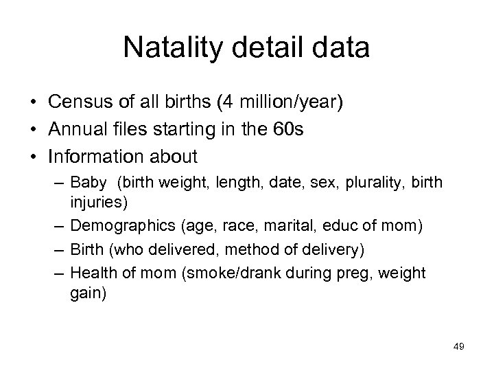
Natality detail data • Census of all births (4 million/year) • Annual files starting in the 60 s • Information about – Baby (birth weight, length, date, sex, plurality, birth injuries) – Demographics (age, race, marital, educ of mom) – Birth (who delivered, method of delivery) – Health of mom (smoke/drank during preg, weight gain) 49
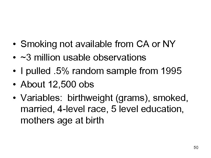
• • • Smoking not available from CA or NY ~3 million usable observations I pulled. 5% random sample from 1995 About 12, 500 obs Variables: birthweight (grams), smoked, married, 4 -level race, 5 level education, mothers age at birth 50
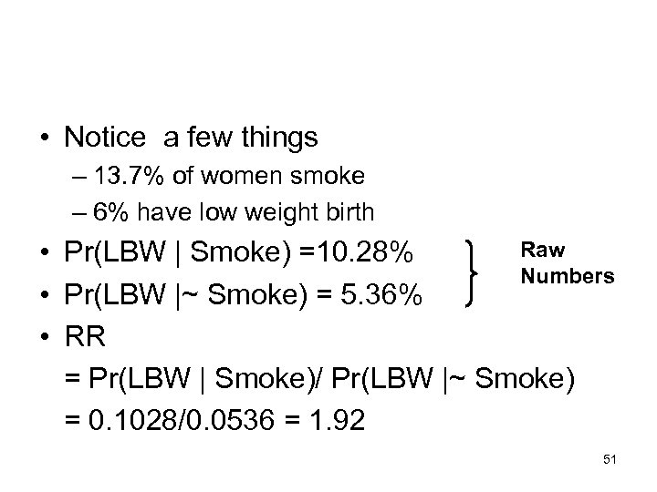
• Notice a few things – 13. 7% of women smoke – 6% have low weight birth Raw • Pr(LBW | Smoke) =10. 28% Numbers • Pr(LBW |~ Smoke) = 5. 36% • RR = Pr(LBW | Smoke)/ Pr(LBW |~ Smoke) = 0. 1028/0. 0536 = 1. 92 51
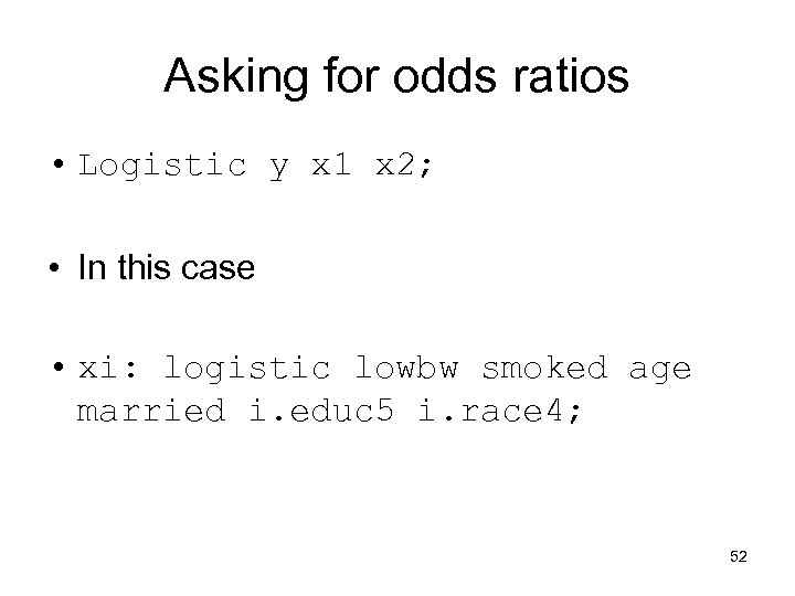
Asking for odds ratios • Logistic y x 1 x 2; • In this case • xi: logistic lowbw smoked age married i. educ 5 i. race 4; 52
![PAR • PAR = (RR – 1) xs /[(1 - xs) + RR xs] PAR • PAR = (RR – 1) xs /[(1 - xs) + RR xs]](https://present5.com/presentation/91ddaef1c419d4510f0534e698f59bba/image-53.jpg)
PAR • PAR = (RR – 1) xs /[(1 - xs) + RR xs] • xs= 0. 137 • RR = 1. 96 • PAR = 0. 116 • 11. 6% of low weight births attributed to maternal smoking 53
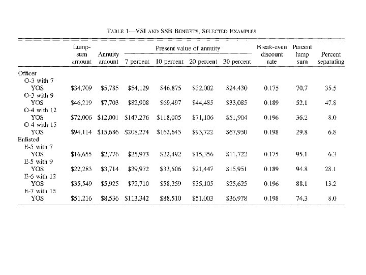
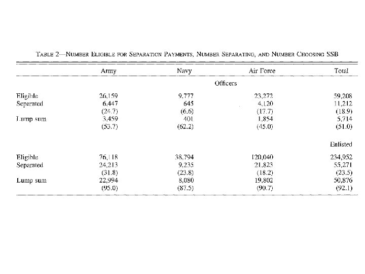
Endowment effect • Ask group to fill out a survey • As a thank you, give them a coffee mug – Have the mug when they fill out the survey • After the survey, offer them a trade of a candy bar for a mug • Reverse the experiment – offer candy bar, then trade for a mug • Comparison sample – give them a choice of mug/candy after survey is complete
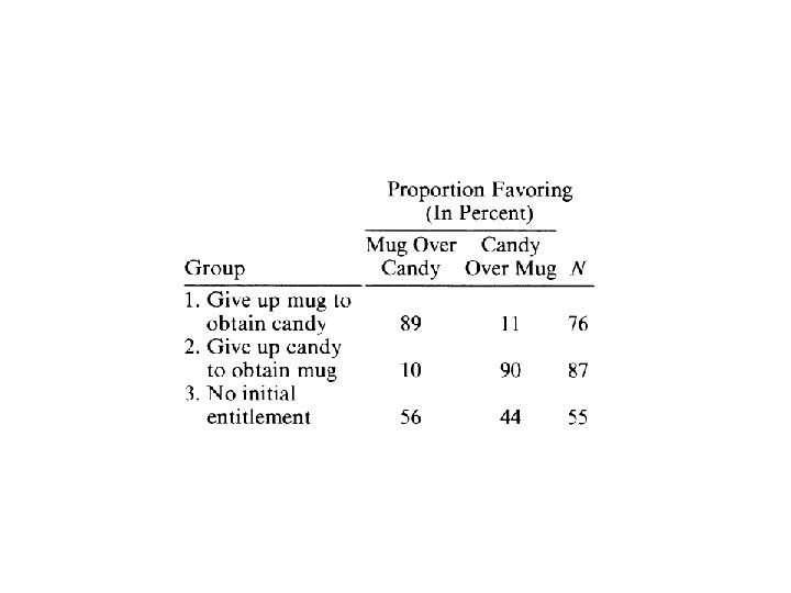
Contrary to simply consumer choice model • Standard util. theory model assume MRS between two good is symmetric • Lack of trading suggests an “endowment” effect – People value the good more once they own it – Generates large discrepancies between WTP and WTA
Policy implications • Example: – A) How much are you willing to pay for clean air? – B) How much do we have to pay you to allow someone to pollute – Answer to B) orders of magnitude larger than A) – Prior – estimate WTP via A and assume equals WTA • Thought of as loss aversion –
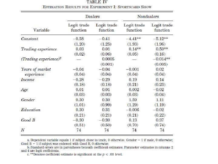
Problem • Artificial situations • Inexperienced may not know value of the item • Solution: see how experienced actors behave when they are endowed with something they can easily value • Two experiments: baseball card shows and collectible pins

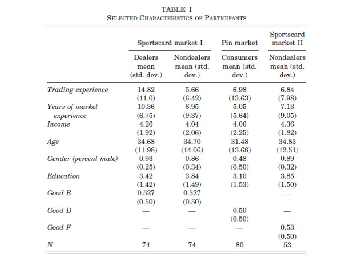
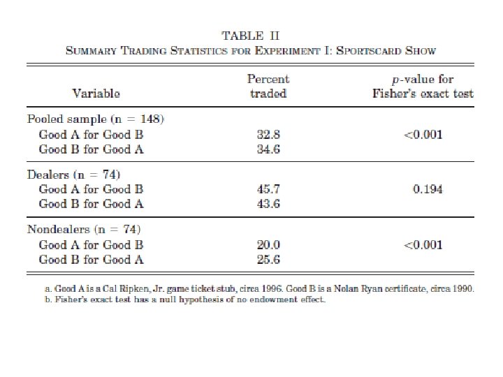
Baseball cards • Two pieces of memorabilia – Game stub from game Cal Ripken Jr set the record for consecutive games played (vs. KC, June 14, 1996) – Certificate commemorating Nolan Ryans’ 300 th win • Ask people to fill out a 5 min survey. In return, they receive one of the pieces, then ask for a trade
91ddaef1c419d4510f0534e698f59bba.ppt