Location Problems John H Vande Vate Spring 2001

Location Problems John H. Vande Vate Spring, 2001 1 1

Outline • Review the Terminal Problem discussed in Daganzo (page 68 -71) • An MIP approach • Rectilinear Location Problems • Euclidean Location Problems • Location - Allocation Problems 2 2

Locating Freight Terminals • Examples: – LTL freight terminals – Public transportation • Local transport to consolidation points – Local collection to freight terminals – Walk to bus stop • Trade-off cost of local transport vs impact on “line haul” – More stops = less local transport – More stops = slower line haul 3 3

Aside • Don’t forget service segmentation! – Express Bus vs Local 4 4

Two-Tier System • LTL depot – shipments consolidated for cross-country transport • Freight terminals – Local shipments are consolidated for delivery to depot • Daily delivery • Single line-haul vehicle 5 5

On a Line • Along a major highway • Along a bus route • . . . 6 6

Question: Freight Terminals? • How many freight terminals should we have and where should we put them? • Costs? – Capital and operating costs of terminals – Local transport cost – Stop Cost –. . . 7 7

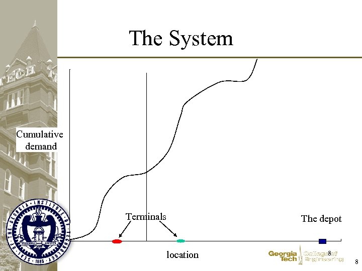
The System Cumulative demand Terminals The depot location 8 8

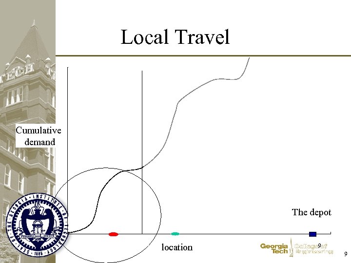
Local Travel Cumulative demand The depot location 9 9

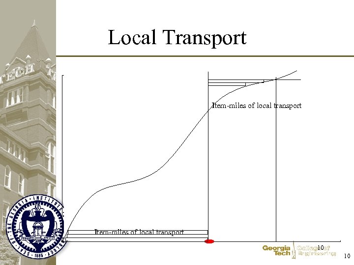
Local Transport Item-miles of local transport 10 10

When is this appropriate? • Walking to the bus stop • Local delivery to freight terminal? • Other suggestions? – Weighted distance – Total distance – Maximum Distance – …. 11 11

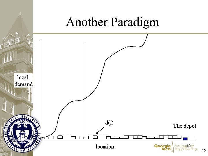
Another Paradigm local demand d(i) location The depot 12 12

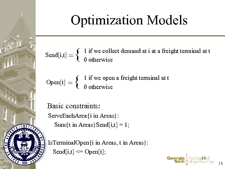
Optimization Models { 1 if we collect demand at i at a freight terminal at t 0 otherwise { 1 if we open a freight terminal at t 0 otherwise Send[i, t] = Open[t] = Basic constraints: Serve. Each. Area{i in Areas}: Sum{t in Areas}Send[i, t] = 1; Is. Terminal. Open{i in Areas, t in Areas}: Send[i, t] <= Open[t]; 13 13

Objectives • Item-miles + Stops sum{a in Areas, t in Areas} d[a]*abs(t-a)*Send[a, t] + sum{t in Areas} stopcost*Open[t]; • Total Distance + Stops sum{a in Areas, t in Areas} abs(t-a)*Send[a, t] + sum{t in Areas} stopcost*Open[t]; 14 14

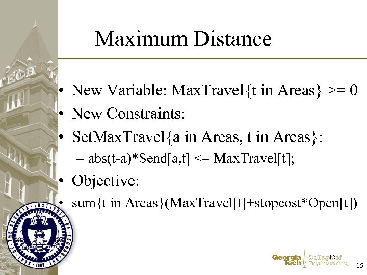
Maximum Distance • New Variable: Max. Travel{t in Areas} >= 0 • New Constraints: • Set. Max. Travel{a in Areas, t in Areas}: – abs(t-a)*Send[a, t] <= Max. Travel[t]; • Objective: • sum{t in Areas}(Max. Travel[t]+stopcost*Open[t]) 15 15

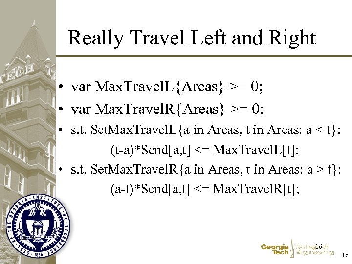
Really Travel Left and Right • var Max. Travel. L{Areas} >= 0; • var Max. Travel. R{Areas} >= 0; • s. t. Set. Max. Travel. L{a in Areas, t in Areas: a < t}: (t-a)*Send[a, t] <= Max. Travel. L[t]; • s. t. Set. Max. Travel. R{a in Areas, t in Areas: a > t}: (a-t)*Send[a, t] <= Max. Travel. R[t]; 16 16

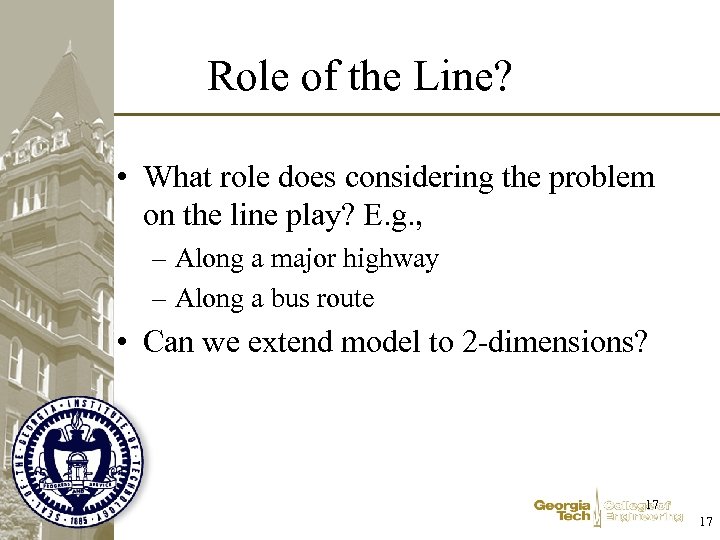
Role of the Line? • What role does considering the problem on the line play? E. g. , – Along a major highway – Along a bus route • Can we extend model to 2 -dimensions? 17 17

Outline • Review the Terminal Problem discussed in Daganzo (page 68 -71) • An MIP approach • Rectilinear Location Problems • Euclidean Location Problems • Location - Allocation Problems 18 18

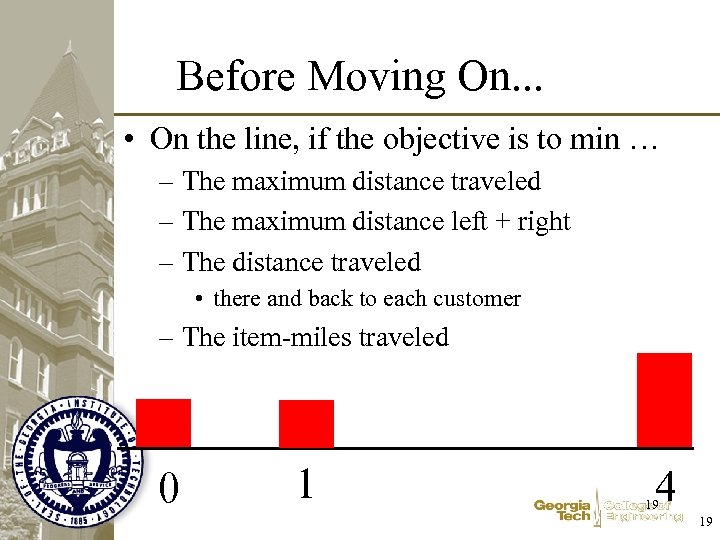
Before Moving On. . . • On the line, if the objective is to min … – The maximum distance traveled – The maximum distance left + right – The distance traveled • there and back to each customer – The item-miles traveled 0 1 4 19 19

Rectilinear Distance • Travel on the streets and avenues • Distance = – number of blocks East-West + – number of blocks North-South • Manhattan Metric • 20 20

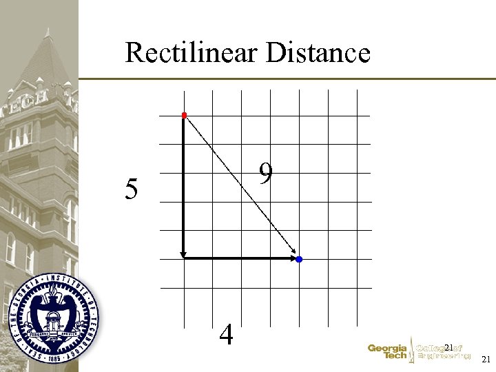
Rectilinear Distance 9 5 4 21 21

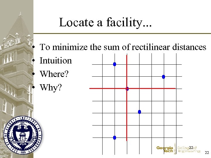
Locate a facility. . . • • To minimize the sum of rectilinear distances Intuition Where? Why? 22 22

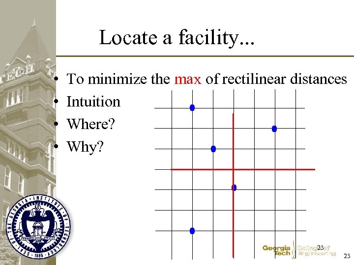
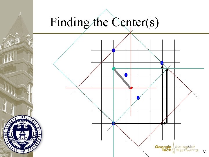
Locate a facility. . . • • To minimize the max of rectilinear distances Intuition Where? Why? 23 23

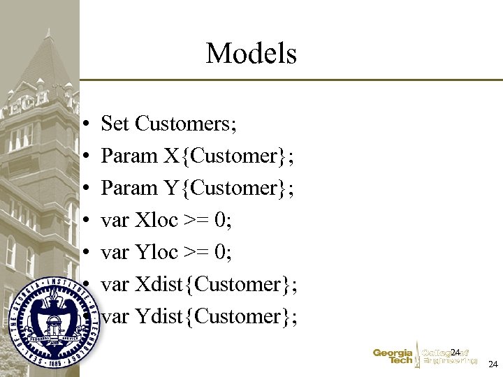
Models • • Set Customers; Param X{Customer}; Param Y{Customer}; var Xloc >= 0; var Yloc >= 0; var Xdist{Customer}; var Ydist{Customer}; 24 24

Constraints • Define. Xdist 1{c in Customer}: Xdist[c] >= X[c]-Xloc; • Define. Xdist 2{c in Customer}: Xdist[c] >= Xloc-X[c]; • Define. Ydist 1{c in Customer}: Ydist[c] >= Y[c]-Yloc; • Define. Ydist 2{c in Customer}: Ydist[c] >= Yloc-Y[c]; 25 25

Objective • Total Distance: – sum{c in Customer}(Xdist[c]+Ydist[c]); • Maximum Distance? 26 26

Minimize The Max? • Var Xloc; • Var Yloc; • Var Xmax >= 0; • var Ymax >= 0; • min objective: Xmax + Ymax; • s. t. Define. Xdist 1{c in Customer}: Xmax >= X[c]-Xloc; • Define. Xdist 2{c in Customer}: Xmax >= Xloc-X[c]; • Define. Ydist 1{c in Customer}: Ymax >= Y[c]-Yloc; • Define. Ydist 2{c in Customer}: Ymax >= Yloc-Y[c]; 27 27

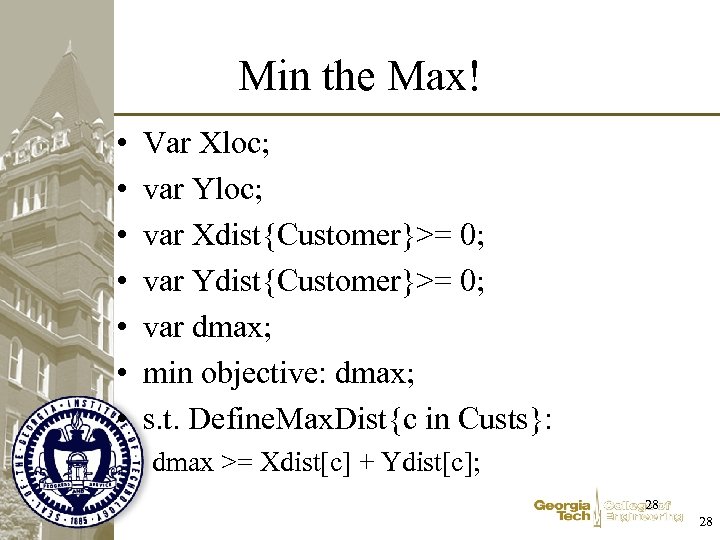
Min the Max! • • Var Xloc; var Yloc; var Xdist{Customer}>= 0; var Ydist{Customer}>= 0; var dmax; min objective: dmax; s. t. Define. Max. Dist{c in Custs}: dmax >= Xdist[c] + Ydist[c]; 28 28

Min the Max Cont’d • Define. Xdist 1{c in Customer}: Xdist[c] >= X[c]-Xloc; • Define. Xdist 2{c in Customer}: Xdist[c] >= Xloc-X[c]; • Define. Ydist 1{c in Customer}: Ydist[c] >= Y[c]-Yloc; • Define. Ydist 2{c in Customer}: Ydist[c] >= Yloc-Y[c]; 29 29

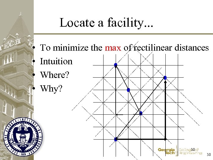
Locate a facility. . . • • To minimize the max of rectilinear distances Intuition Where? Why? 30 30

Finding the Center(s) 31 31

Assignment #1 • • • NIMBY…. Maximize the Minimum Distance Can’t say Xdist[c] <= X[c] - Xloc; Come up with a good formulation FOR DISCUSSION IN CLASS NEXT TIME 32 32

Outline • Review the Terminal Problem discussed in Daganzo (page 68 -71) • An MIP approach • Rectilinear Location Problems • Euclidean Location Problems • Location - Allocation Problems 33 33

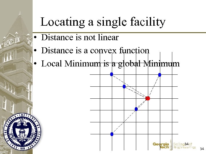
Locating a single facility • Distance is not linear • Distance is a convex function • Local Minimum is a global Minimum 34 34

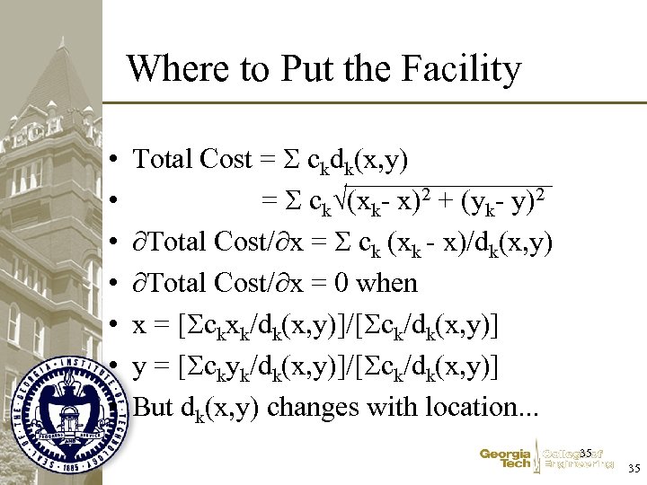
Where to Put the Facility • • Total Cost = S ckdk(x, y) = S ck (xk- x)2 + (yk- y)2 Total Cost/ x = S ck (xk - x)/dk(x, y) Total Cost/ x = 0 when x = [Sckxk/dk(x, y)]/[Sck/dk(x, y)] y = [Sckyk/dk(x, y)]/[Sck/dk(x, y)] But dk(x, y) changes with location. . . 35 35

Iterative Strategy • Start somewhere, e. g. , – x = [Sckxk]/[Sck] – y = [Sckyk]/[Sck] – as though dk= 1. • Step 1: Calculate values of dk • Step 2: Refine values of x and y – x = [Sckxk/dk]/[Sck/dk] – y = [Sckyk/dk]/[Sck/dk] • Repeat Steps 1 and 2. . 36 36

Convex Minimization • Call on Convex Minimization Tool • Minos, Interior Point Methods, … • Typically don’t support discrete variables too… 37 37

Locating Several Facilities • Fixed Number of Facilities to Consider • Single Sourcing • Two Questions: – Location: Where – Allocation: Whom to serve • Each is simple • Together they are “harder” 38 38

Iterative Approach • Put the facilities somewhere • Step 1: Assign the Customers to the Facilities • Step 2: Find the best location for each facility given the assignments (see previous method) • Repeat Step 1 and Step 2 …. 39 39

Assign Customers to Facilities • Uncapacitated (facilities can be any size) – “Greedy”: Assign each customer to closest facility • Capacitated – Use Optimization 40 40

Allocation Model Var x{Custs, Facs} binary; minimize Allocation. Cost: sum{c in Custs, f in Facs} C[c, f]*x[c, f]; s. t. Assign. Each. Cust{c in Custs}: sum{f in Facs} x[c, f] = 1; s. t. Facility. Capacity{f in Facs}: sum{c in Custs}D[c]*c[c, f] <= Cap[f]; 41 41

The Rest of the Story • If there is – Value Added: E. g. , BMW Assembly Plant – High Value items: E. g. , Intel EU distribution center • If there is labor content… • Competition… • Service vs Cost. . . 42 42