Local Sparsification for Scalable Module Identification in Networks

Local Sparsification for Scalable Module Identification in Networks Srinivasan Parthasarathy Joint work with V. Satuluri, Y. Ruan, D. Fuhry, Y. Zhang Data Mining Research Laboratory Dept. of Computer Science and Engineering The Ohio State University 1

The Data Deluge “Every 2 days we create as much information as we did up to 2003” - Eric Schmidt, Google ex-CEO 2

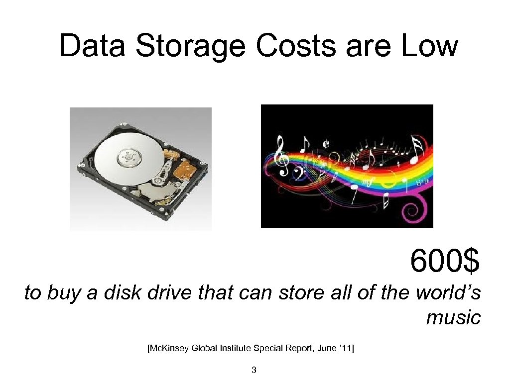
Data Storage Costs are Low 600$ to buy a disk drive that can store all of the world’s music [Mc. Kinsey Global Institute Special Report, June ’ 11] 3

Data does not exist in isolation. 4

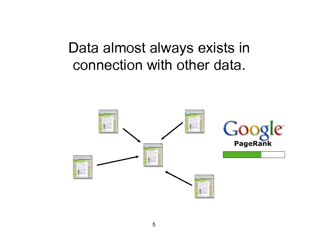
Data almost always exists in connection with other data. 5

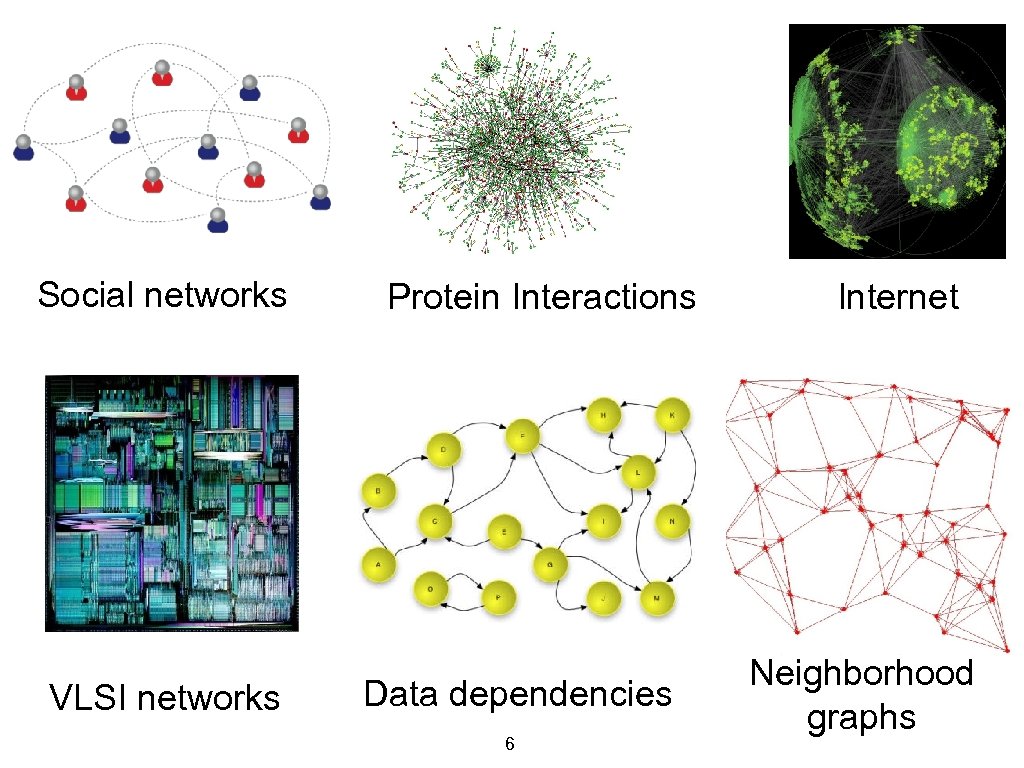
Social networks VLSI networks Protein Interactions Data dependencies 6 Internet Neighborhood graphs

All this data is only useful if we can scalably extract useful knowledge 7

Challenges 1. Large Scale Billion-edge graphs commonplace Scalable solutions are needed 8

Challenges 2. Noise Links on the web, protein interactions Need to alleviate 9

Challenges 3. Novel structure Hub nodes, small world phenomena, clusters of varying densities and sizes, directionality Novel algorithms or techniques are needed 10

Challenges 4. Domain Specific Needs E. g. Balance, Constraints etc. Need mechanisms to specify 11

Challenges 5. Network Dynamics How do communities evolve? Which actors have influence? How do clusters change as a function of external factors? 12

Challenges 6. Cognitive Overload Need to support guided interaction for human in the loop 13

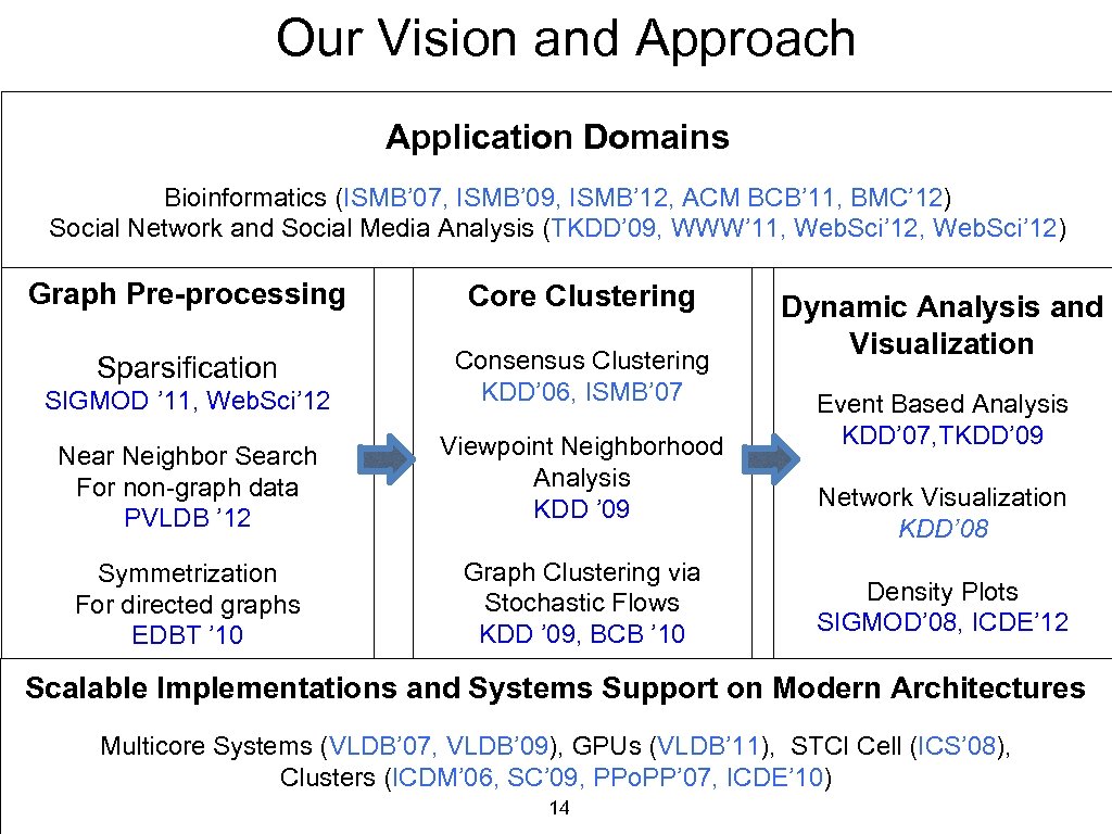
Our Vision and Approach Application Domains Bioinformatics (ISMB’ 07, ISMB’ 09, ISMB’ 12, ACM BCB’ 11, BMC’ 12) Social Network and Social Media Analysis (TKDD’ 09, WWW’ 11, Web. Sci’ 12) Graph Pre-processing Core Clustering Sparsification SIGMOD ’ 11, Web. Sci’ 12 Consensus Clustering KDD’ 06, ISMB’ 07 Near Neighbor Search For non-graph data PVLDB ’ 12 Viewpoint Neighborhood Analysis KDD ’ 09 Symmetrization For directed graphs EDBT ’ 10 Graph Clustering via Stochastic Flows KDD ’ 09, BCB ’ 10 Dynamic Analysis and Visualization Event Based Analysis KDD’ 07, TKDD’ 09 Network Visualization KDD’ 08 Density Plots SIGMOD’ 08, ICDE’ 12 Scalable Implementations and Systems Support on Modern Architectures Multicore Systems (VLDB’ 07, VLDB’ 09), GPUs (VLDB’ 11), STCI Cell (ICS’ 08), Clusters (ICDM’ 06, SC’ 09, PPo. PP’ 07, ICDE’ 10) 14

Graph Sparsification for Community Discovery SIGMOD ’ 11, Web. Sci’ 12 15

Is there a simple pre-processing of the graph to reduce the edge set that can “clarify” or “simplify” its cluster structure? 16

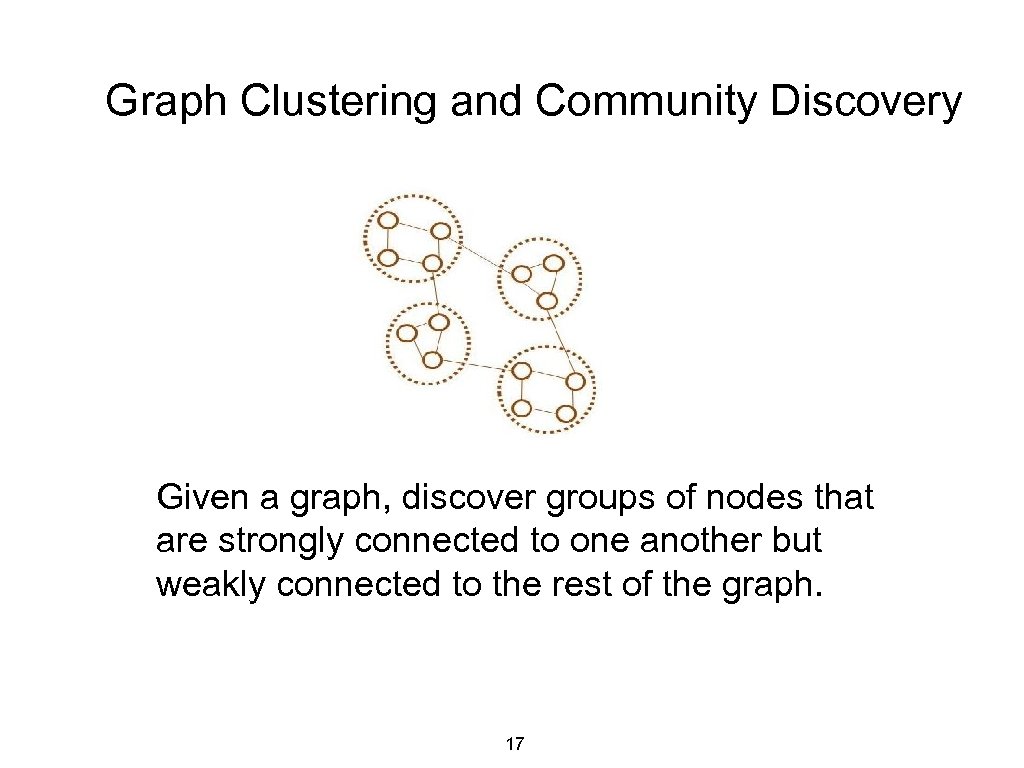
Graph Clustering and Community Discovery Given a graph, discover groups of nodes that are strongly connected to one another but weakly connected to the rest of the graph. 17

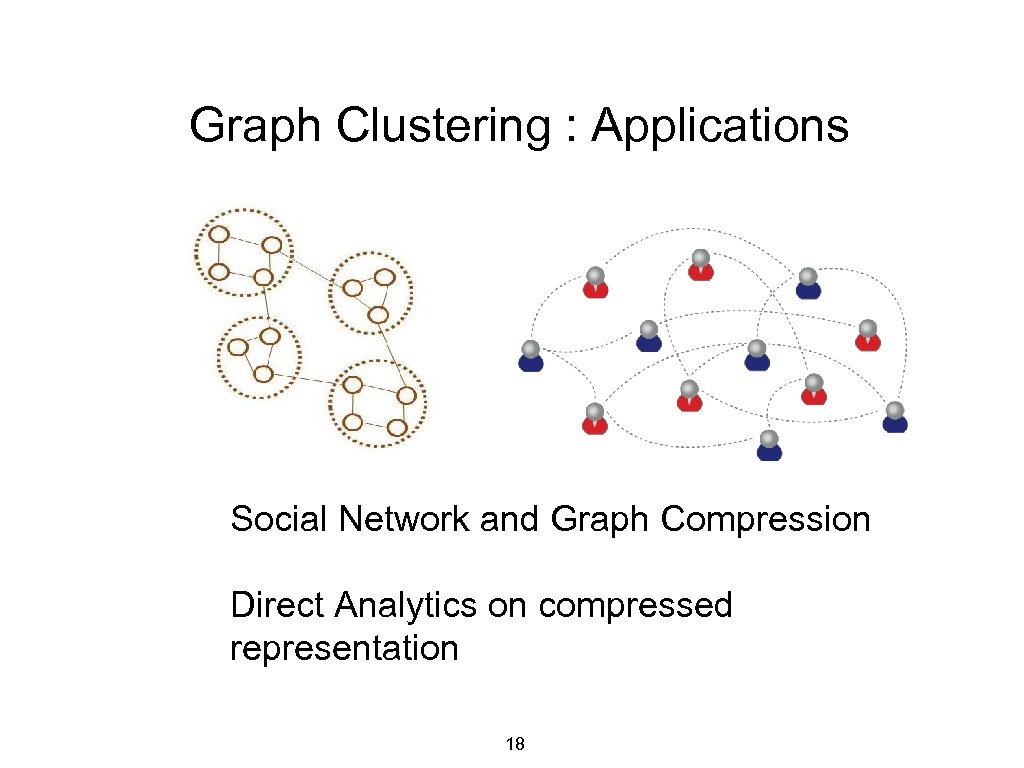
Graph Clustering : Applications Social Network and Graph Compression Direct Analytics on compressed representation 18

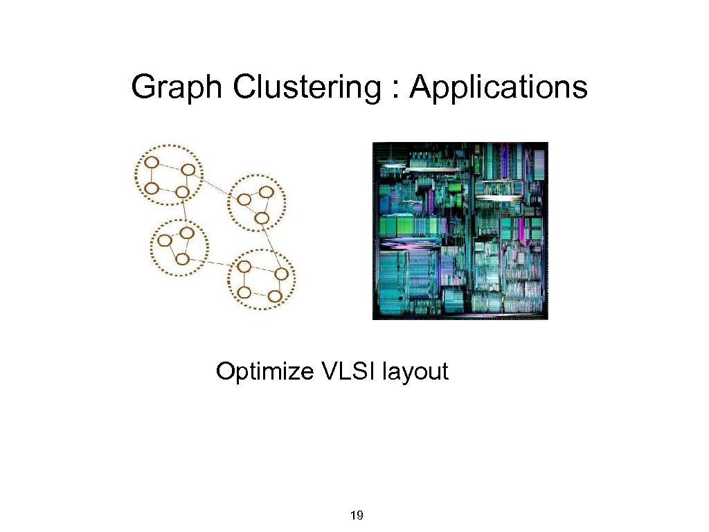
Graph Clustering : Applications Optimize VLSI layout 19

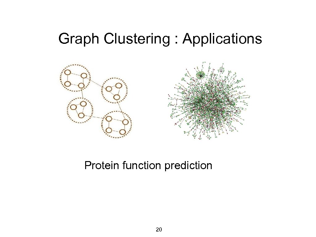
Graph Clustering : Applications Protein function prediction 20

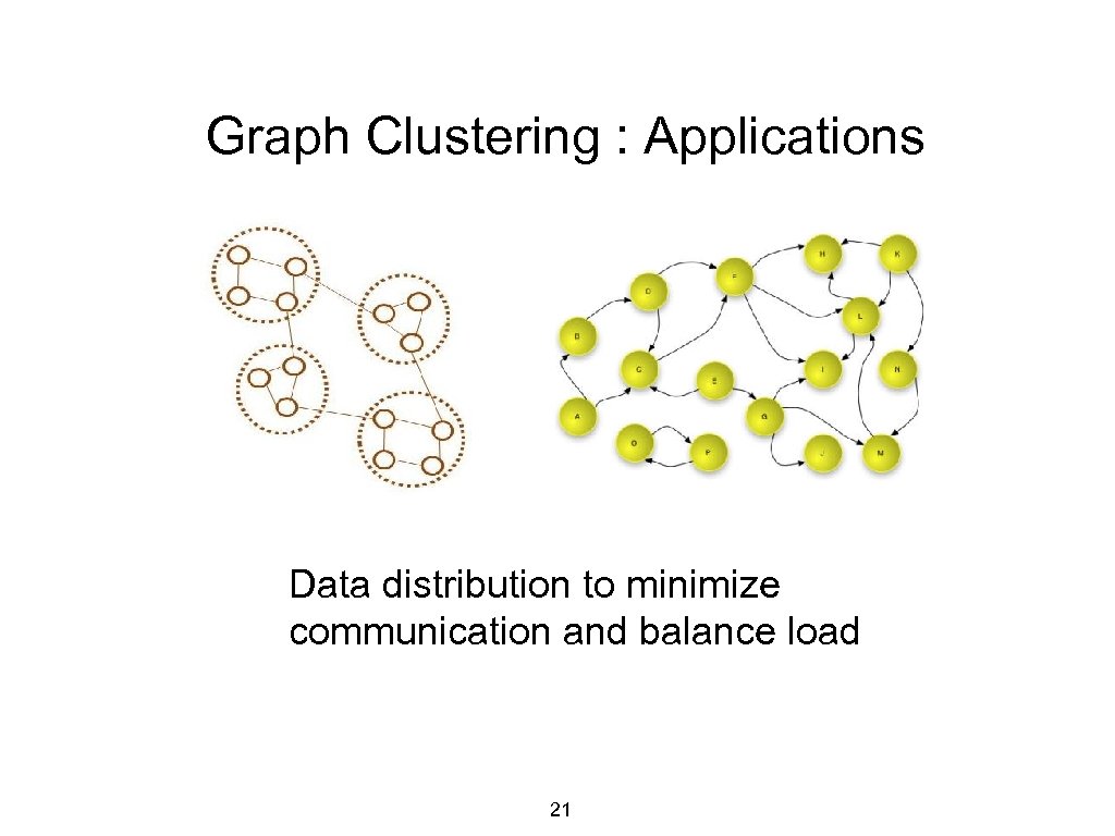
Graph Clustering : Applications Data distribution to minimize communication and balance load 21

Is there a simple pre-processing of the graph to reduce the edge set that can “clarify” or “simplify” its cluster structure? 22

Preview Original Sparsified [Automatically visualized using Prefuse] 23

The promise Clustering algorithms can run much faster and be more accurate on a sparsified graph. Ditto for Network Visualization 24

Utopian Objective Retain edges which are likely to be intra-cluster edges, while discarding likely inter-cluster edges. 25

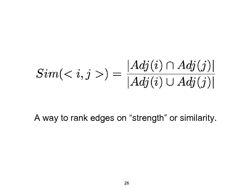
A way to rank edges on “strength” or similarity. 26

Algorithm: Global Sparsification (G-Spar) Parameter: Sparsification ratio, s 1. For each edge <i, j>: (i) Calculate Sim ( <i, j> ) 2. Retain top s% of edges in order of Sim, discard others 27

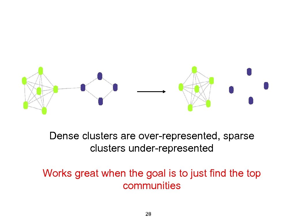
Dense clusters are over-represented, sparse clusters under-represented Works great when the goal is to just find the top communities 28

Algorithm: Local Sparsification (L-Spar) Parameter: Sparsification exponent, e (0 < e < 1) 1. For each node i of degree di: (i) For each neighbor j: (a) Calculate Sim ( <i, j> ) (ii) Retain top (d i)e neighbors in order of Sim, for node i Underscoring the importance of Local Ranking 29

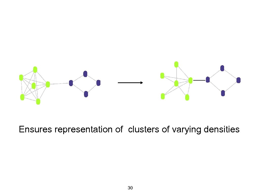
Ensures representation of clusters of varying densities 30

But. . . Similarity computation is expensive! 31

A randomized, approximate solution based on Minwise Hashing [Broder et. al. , 1998] 32

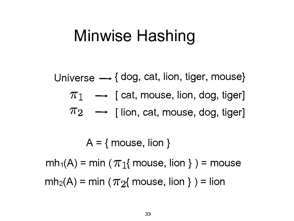
Minwise Hashing Universe { dog, cat, lion, tiger, mouse} [ cat, mouse, lion, dog, tiger] [ lion, cat, mouse, dog, tiger] A = { mouse, lion } mh 1(A) = min ( { mouse, lion } ) = mouse mh 2(A) = min ( { mouse, lion } ) = lion 33

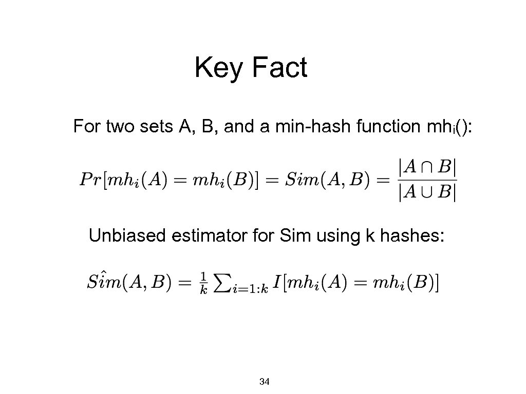
Key Fact For two sets A, B, and a min-hash function mhi(): Unbiased estimator for Sim using k hashes: 34

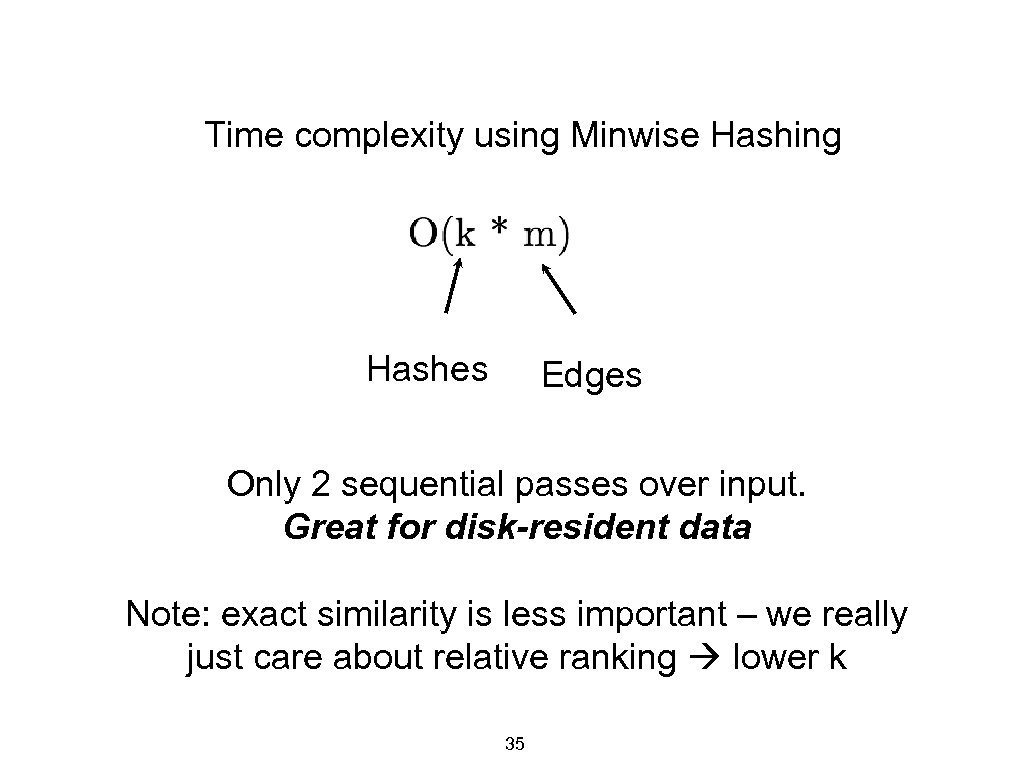
Time complexity using Minwise Hashing Hashes Edges Only 2 sequential passes over input. Great for disk-resident data Note: exact similarity is less important – we really just care about relative ranking lower k 35

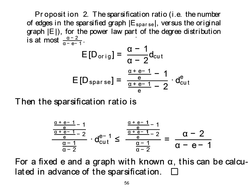
• • Theoretical Analysis of L-Spar: Main Results Q: Why choose top de edges for a node of degree d? • A: Conservatively sparsify low-degree nodes, aggressively sparsify hub nodes. Easy to control degree of sparsification. Proposition: If input graph has power-law degree distn. with exponent , then sparsified graph also has power-law degree distn. with exponent Corollary: The sparsification ratio corresponding to exponent e is no more than For = 2. 1 and e = 0. 5, ~17% edges will be retained. • Higher (steeper power-laws) and/or lower e leads to more sparsification.

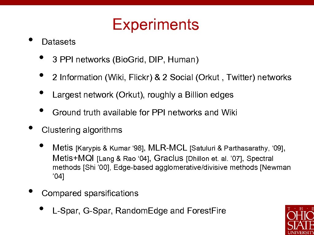
• Experiments Datasets • • • 3 PPI networks (Bio. Grid, DIP, Human) 2 Information (Wiki, Flickr) & 2 Social (Orkut , Twitter) networks Largest network (Orkut), roughly a Billion edges Ground truth available for PPI networks and Wiki Clustering algorithms • Metis [Karypis & Kumar ‘ 98], MLR-MCL [Satuluri & Parthasarathy, ‘ 09], Metis+MQI [Lang & Rao ‘ 04], Graclus [Dhillon et. al. ’ 07], Spectral methods [Shi ’ 00], Edge-based agglomerative/divisive methods [Newman ’ 04] • Compared sparsifications • L-Spar, G-Spar, Random. Edge and Forest. Fire

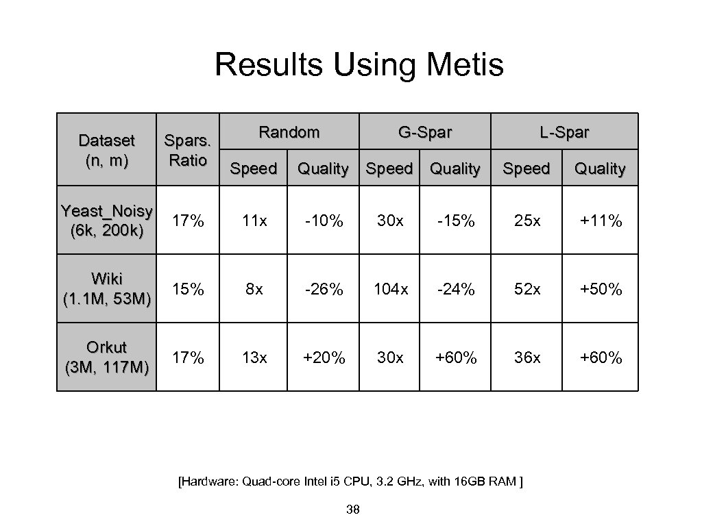
Results Using Metis Random G-Spar Dataset (n, m) Spars. Ratio Yeast_Noisy (6 k, 200 k) 17% 11 x -10% 30 x Wiki (1. 1 M, 53 M) 15% 8 x -26% Orkut (3 M, 117 M) 17% 13 x +20% Speed Quality L-Spar Speed Quality -15% 25 x +11% 104 x -24% 52 x +50% 30 x +60% 36 x +60% [Hardware: Quad-core Intel i 5 CPU, 3. 2 GHz, with 16 GB RAM ] 38

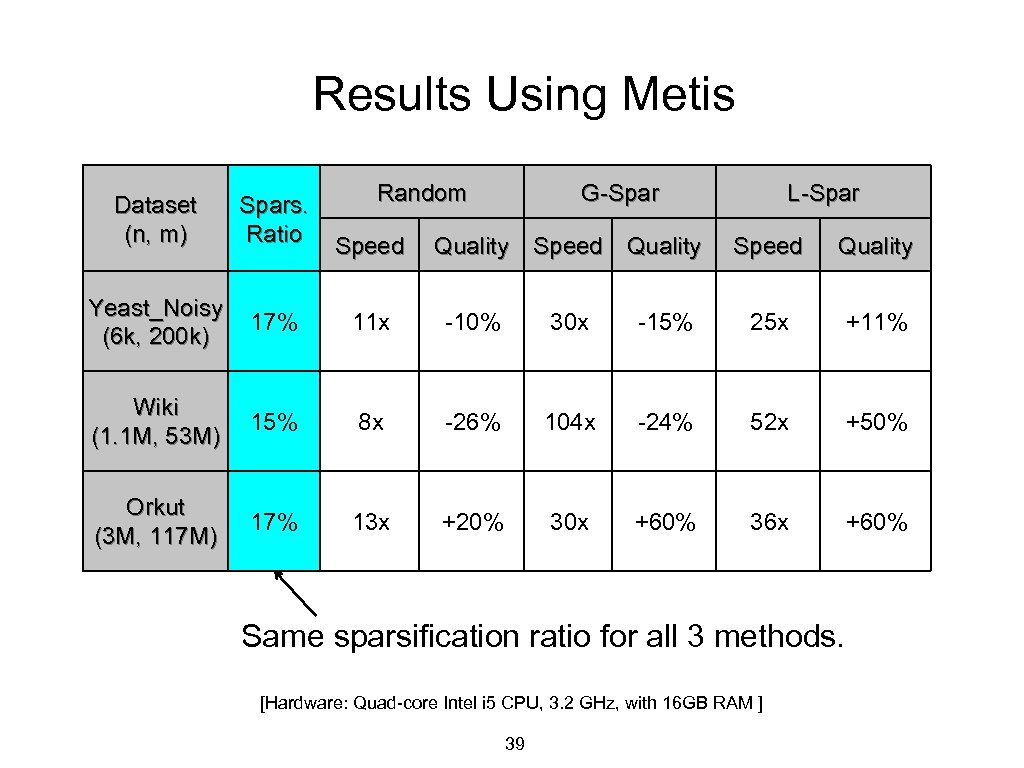
Results Using Metis Random G-Spar Dataset (n, m) Spars. Ratio Yeast_Noisy (6 k, 200 k) 17% 11 x -10% 30 x Wiki (1. 1 M, 53 M) 15% 8 x -26% Orkut (3 M, 117 M) 17% 13 x +20% Speed Quality L-Spar Speed Quality -15% 25 x +11% 104 x -24% 52 x +50% 30 x +60% 36 x +60% Same sparsification ratio for all 3 methods. [Hardware: Quad-core Intel i 5 CPU, 3. 2 GHz, with 16 GB RAM ] 39

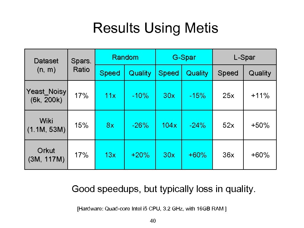
Results Using Metis Random G-Spar Dataset (n, m) Spars. Ratio Yeast_Noisy (6 k, 200 k) 17% 11 x -10% 30 x Wiki (1. 1 M, 53 M) 15% 8 x -26% Orkut (3 M, 117 M) 17% 13 x +20% Speed Quality L-Spar Speed Quality -15% 25 x +11% 104 x -24% 52 x +50% 30 x +60% 36 x +60% Good speedups, but typically loss in quality. [Hardware: Quad-core Intel i 5 CPU, 3. 2 GHz, with 16 GB RAM ] 40

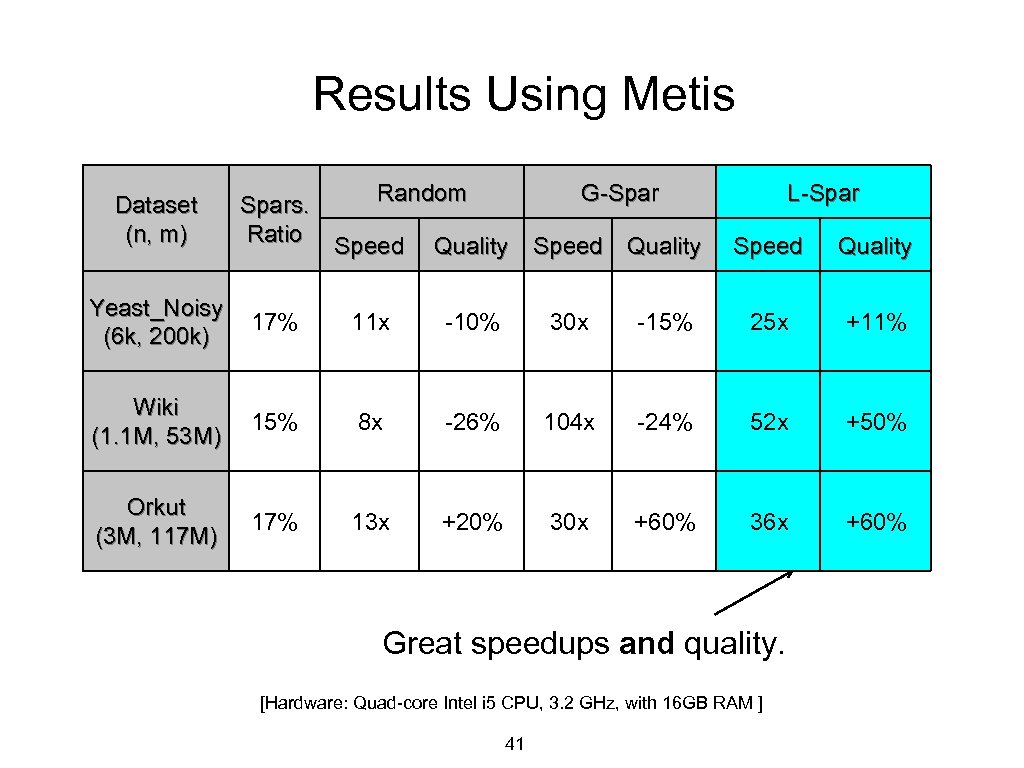
Results Using Metis Random G-Spar Dataset (n, m) Spars. Ratio Yeast_Noisy (6 k, 200 k) 17% 11 x -10% 30 x Wiki (1. 1 M, 53 M) 15% 8 x -26% Orkut (3 M, 117 M) 17% 13 x +20% Speed Quality L-Spar Speed Quality -15% 25 x +11% 104 x -24% 52 x +50% 30 x +60% 36 x +60% Great speedups and quality. [Hardware: Quad-core Intel i 5 CPU, 3. 2 GHz, with 16 GB RAM ] 41

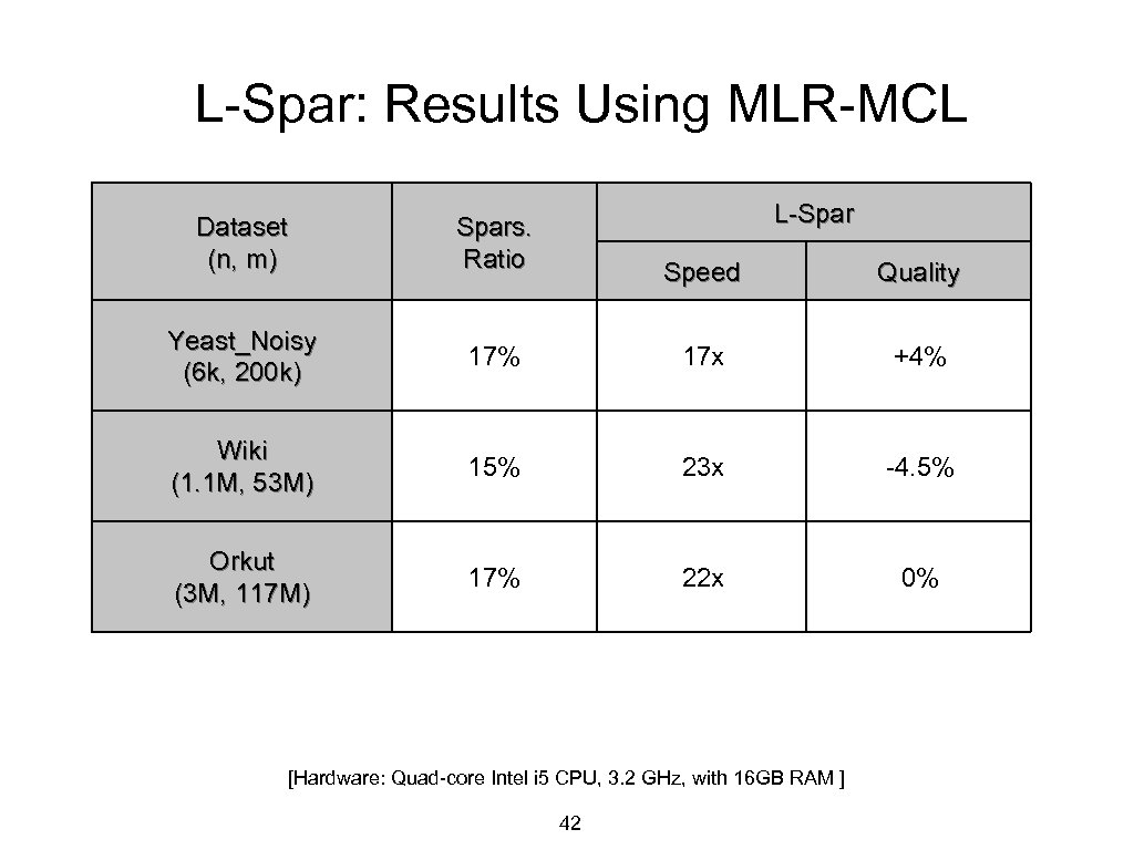
L-Spar: Results Using MLR-MCL Dataset (n, m) Yeast_Noisy (6 k, 200 k) L-Spars. Ratio Speed Quality 17% 17 x +4% Wiki (1. 1 M, 53 M) 15% 23 x -4. 5% Orkut (3 M, 117 M) 17% 22 x 0% [Hardware: Quad-core Intel i 5 CPU, 3. 2 GHz, with 16 GB RAM ] 42

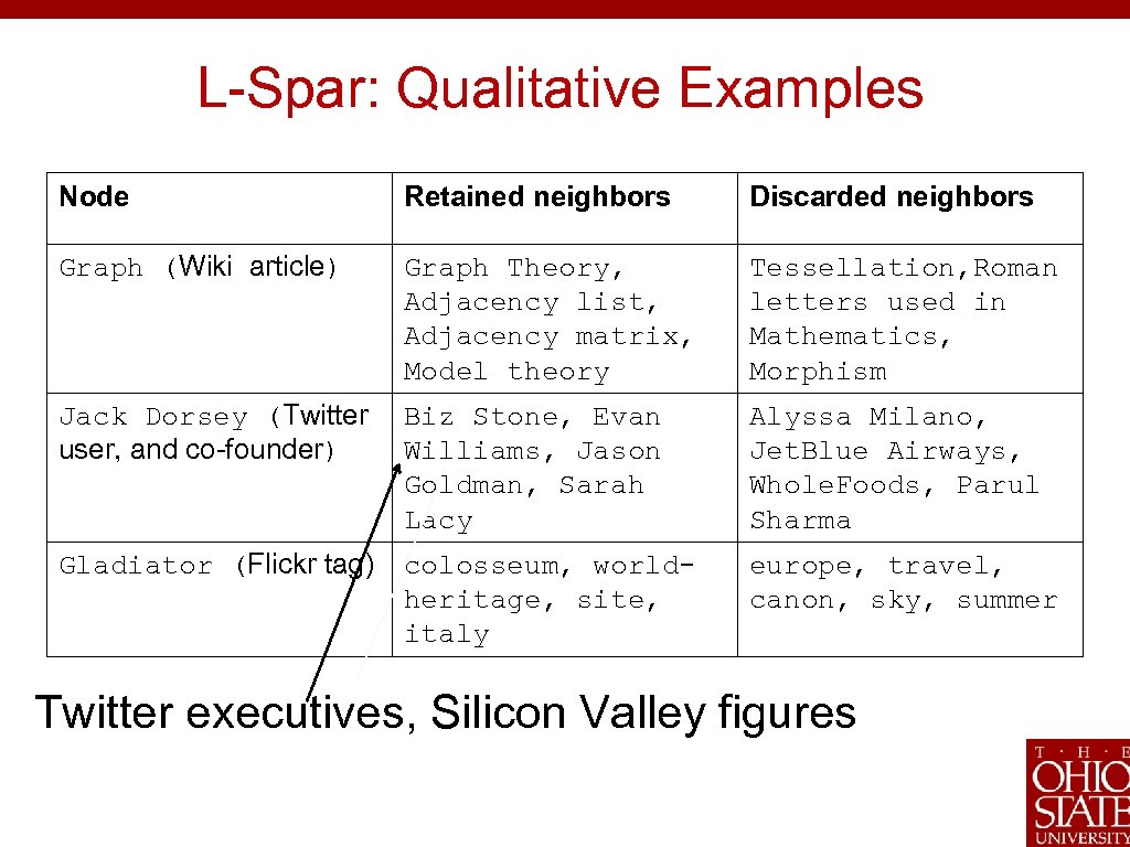
L-Spar: Qualitative Examples Node Retained neighbors Discarded neighbors Graph (Wiki article) Graph Theory, Adjacency list, Adjacency matrix, Model theory Tessellation, Roman letters used in Mathematics, Morphism Jack Dorsey (Twitter user, and co-founder) Biz Stone, Evan Williams, Jason Goldman, Sarah Lacy Alyssa Milano, Jet. Blue Airways, Whole. Foods, Parul Sharma Gladiator (Flickr tag) colosseum, worldheritage, site, italy europe, travel, canon, sky, summer Twitter executives, Silicon Valley figures

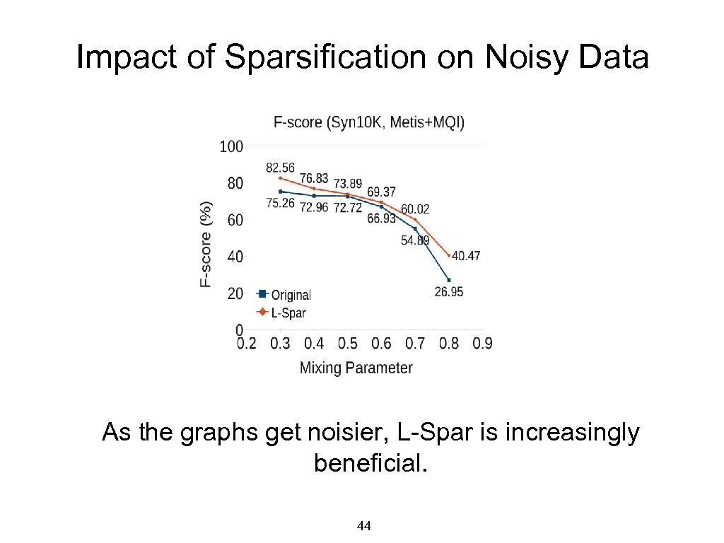
Impact of Sparsification on Noisy Data As the graphs get noisier, L-Spar is increasingly beneficial. 44

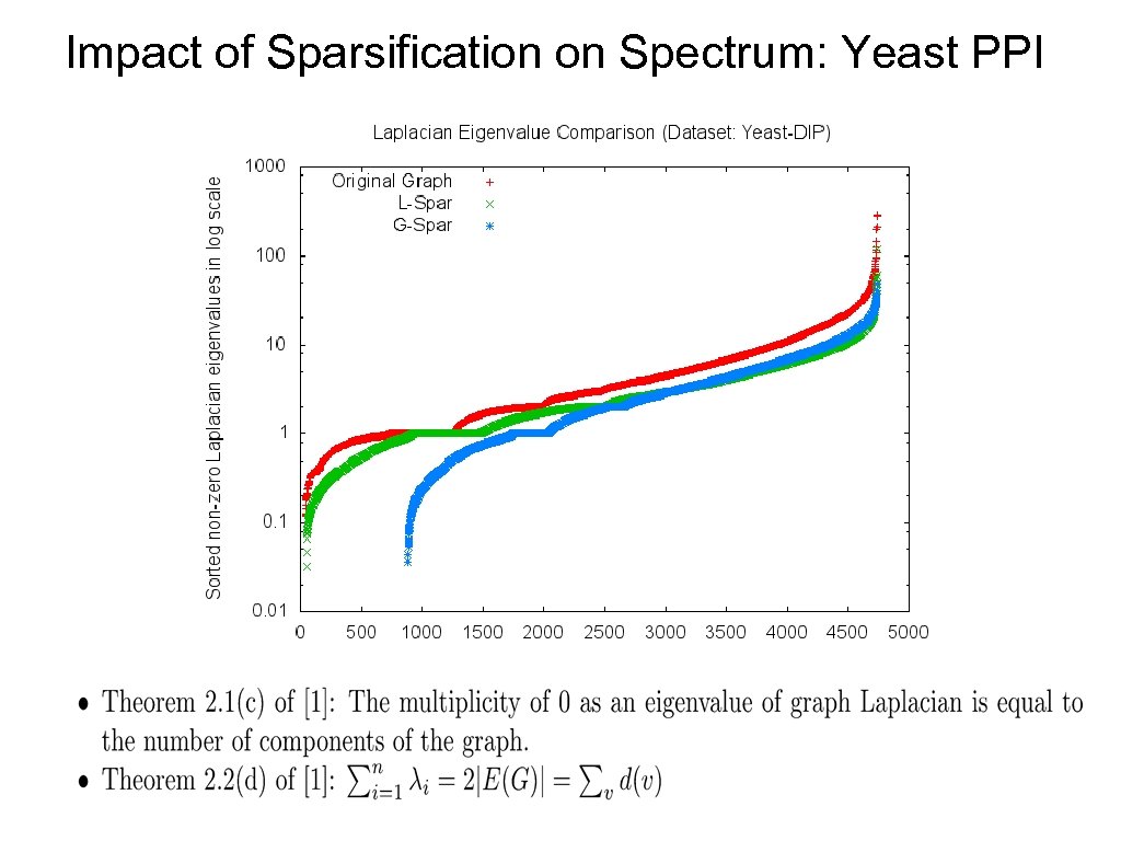
Impact of Sparsification on Spectrum: Yeast PPI

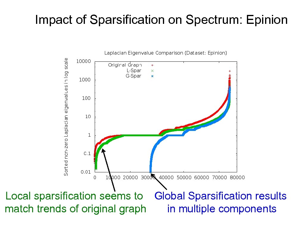
Impact of Sparsification on Spectrum: Epinion Local sparsification seems to Global Sparsification results match trends of original graph in multiple components

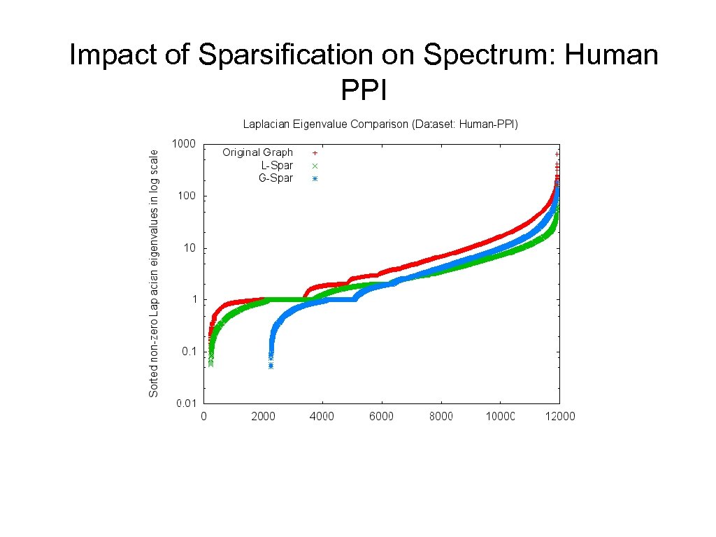
Impact of Sparsification on Spectrum: Human PPI

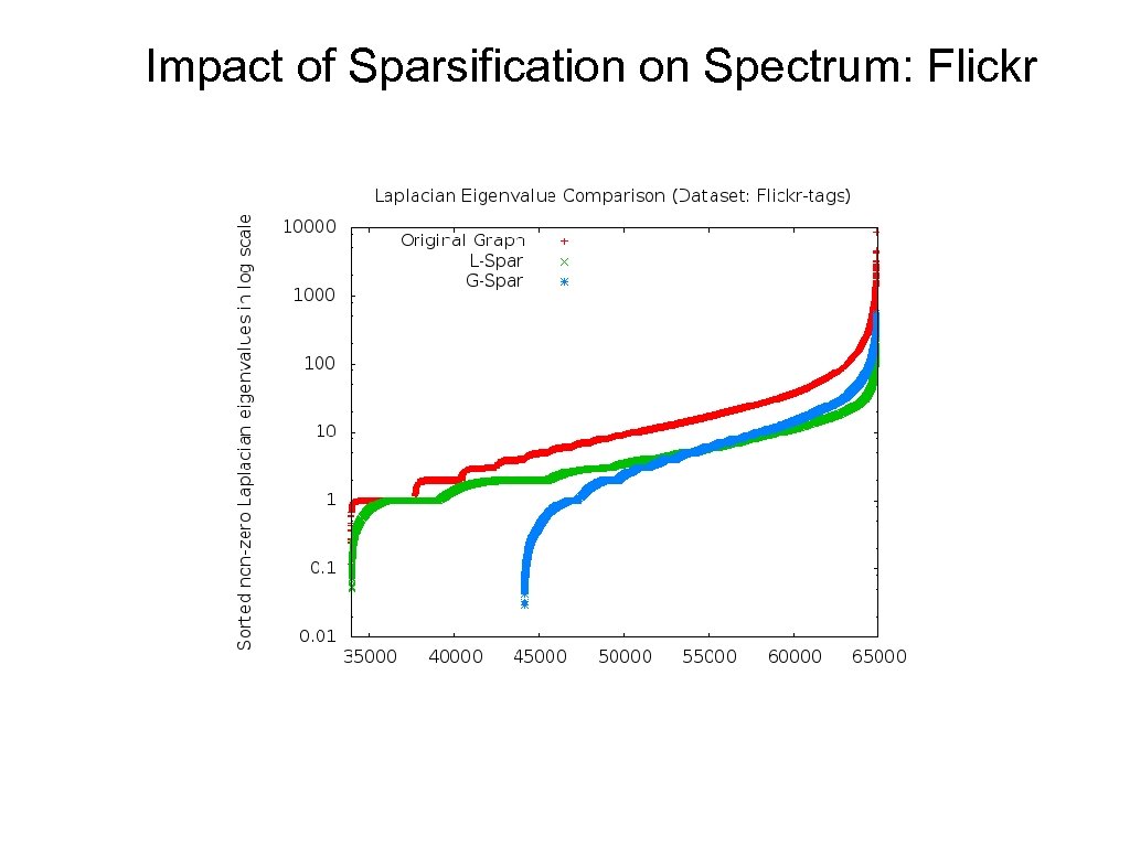
Impact of Sparsification on Spectrum: Flickr

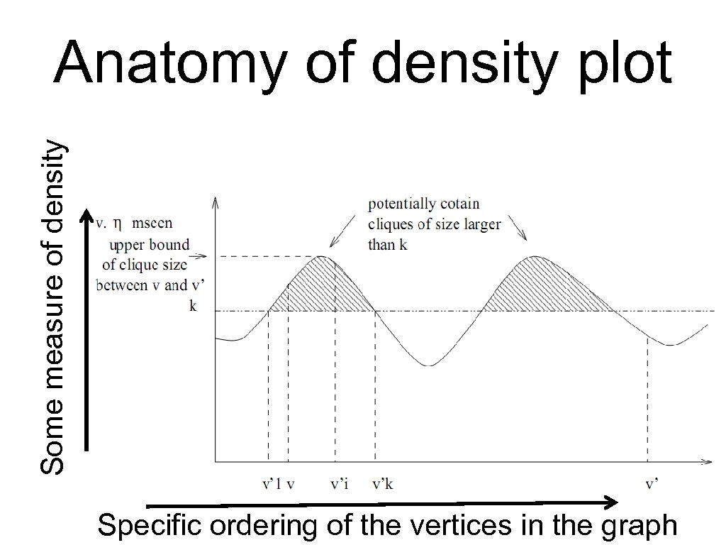
Some measure of density Anatomy of density plot Specific ordering of 49 vertices in the graph the

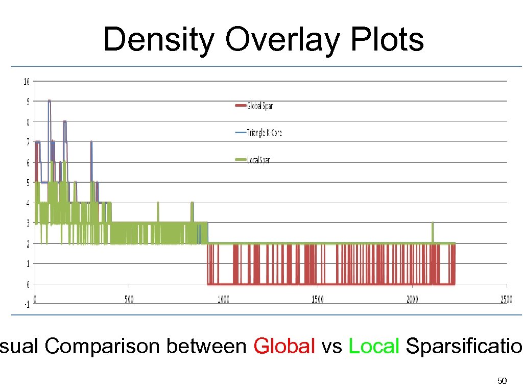
Density Overlay Plots sual Comparison between Global vs Local Sparsification 50

Summary Sparsification: Simple pre-processing that makes a big difference • • • Only tens of seconds to execute on multi-million-node graphs. Reduces clustering time from hours down to minutes. Improves accuracy by removing noisy edges for several algorithms. Helps visualization Ongoing and future work • • Spectral results suggests one might be able to provide theoretical rationale – Can we tease it out? Investigate other kinds of graphs, incorporating content, novel applications (e. g. wireless sensor networks, VLSI design) 51

Prior Work • Random edge Sampling [Karger ‘ 94] • Sampling in proportion to effective resistances: good guarantees but very slow [Spielman and Srivastava ‘ 08] • Matrix sparsification : Fast, but same as random sampling in the absence of weights. [Arora et. al. ’ 06] 52

Topological Measures 53

$Modularity (from Wikipedia ) • Modularity is the fraction of the edges that fall$

Modularity (from Wikipedia ) • Modularity is the fraction of the edges that fall within the given groups minus the expected such fraction if edges were distributed at random. The value of the modularity lies in the range [− 1/2, 1). It is positive if the number of edges within groups exceeds the number expected on the basis of chance. 54

55

56

The MCL algorithm Input: A, Adjacency matrix Initialize M to MG, the canonical transition matrix M: = MG: = (A+I) D-1 Enhances flow to well-connected nodes (i. e. nodes within a community). Expand: M : = M*M Inflate: M : = M. ^r (r usually 2), renormalize columns Increases inequality in each column. “Rich get richer, poor get poorer. ” (reduces flow across communities) Prune Converged? Yes Output clusters No Saves memory by removing entries close to zero. Enables faster convergence Clustering Interpretation: Nodes flowing into the same sink node are assigned same cluster labels