LECTURES 9 — 11 Exchange rates in the

LECTURES 9 - 11 Exchange rates in the short run

Introduction • Substantial deviations from purchasing power parity (PPP) occur in the short run: the same basket of goods generally does not cost the same everywhere at all times. • These short-run failures of the monetary approach prompted economists to develop an alternative theory to explain exchange rates in the short run: the asset approach to exchange rates. • The asset approach is based on the idea that currencies are assets. • The price of the asset in this case is the spot exchange rate, the price of one unit of foreign exchange.

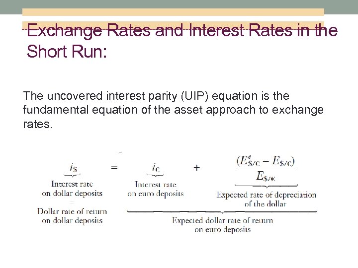Exchange Rates and Interest Rates in the Short Run: The uncovered interest parity (UIP) equation is the fundamental equation of the asset approach to exchange rates.

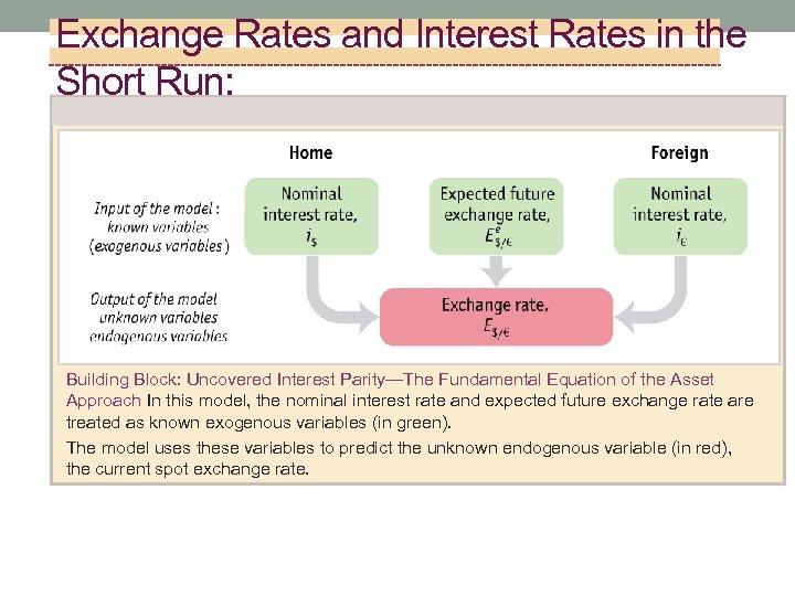Exchange Rates and Interest Rates in the Short Run: Building Block: Uncovered Interest Parity—The Fundamental Equation of the Asset Approach In this model, the nominal interest rate and expected future exchange rate are treated as known exogenous variables (in green). The model uses these variables to predict the unknown endogenous variable (in red), the current spot exchange rate.

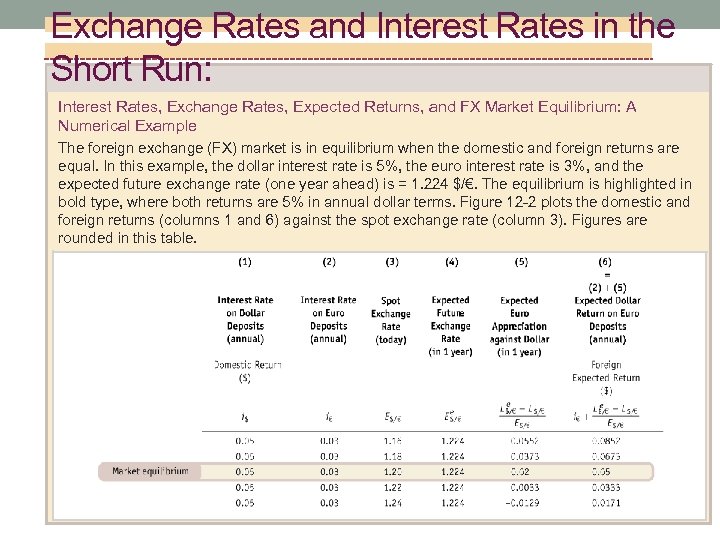Exchange Rates and Interest Rates in the Short Run: Interest Rates, Exchange Rates, Expected Returns, and FX Market Equilibrium: A Numerical Example The foreign exchange (FX) market is in equilibrium when the domestic and foreign returns are equal. In this example, the dollar interest rate is 5%, the euro interest rate is 3%, and the expected future exchange rate (one year ahead) is = 1. 224 $/€. The equilibrium is highlighted in bold type, where both returns are 5% in annual dollar terms. Figure 12 -2 plots the domestic and foreign returns (columns 1 and 6) against the spot exchange rate (column 3). Figures are rounded in this table.

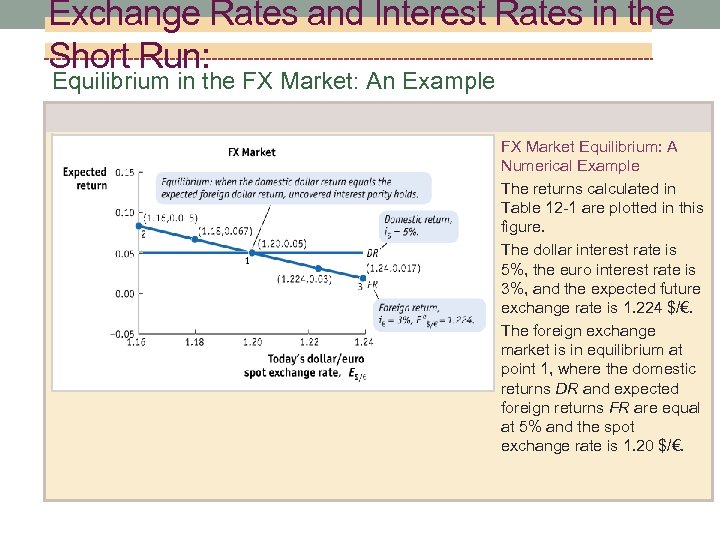Exchange Rates and Interest Rates in the Short Run: Equilibrium in the FX Market: An Example FX Market Equilibrium: A Numerical Example The returns calculated in Table 12 -1 are plotted in this figure. The dollar interest rate is 5%, the euro interest rate is 3%, and the expected future exchange rate is 1. 224 $/€. The foreign exchange market is in equilibrium at point 1, where the domestic returns DR and expected foreign returns FR are equal at 5% and the spot exchange rate is 1. 20 $/€.

Exchange Rates and Interest Rates in the Short Run: Changes in Domestic and Foreign Returns and FX Market Equilibrium To gain greater familiarity with the model, let’s see how the FX market example shown in the previous figure responds to three separate shocks: ■ A higher domestic interest rate, i$ = 7% ■ A lower foreign interest rate, i€ = 1% ■ A lower expected future exchange rate, Ee$/€ = 1. 20 $/€

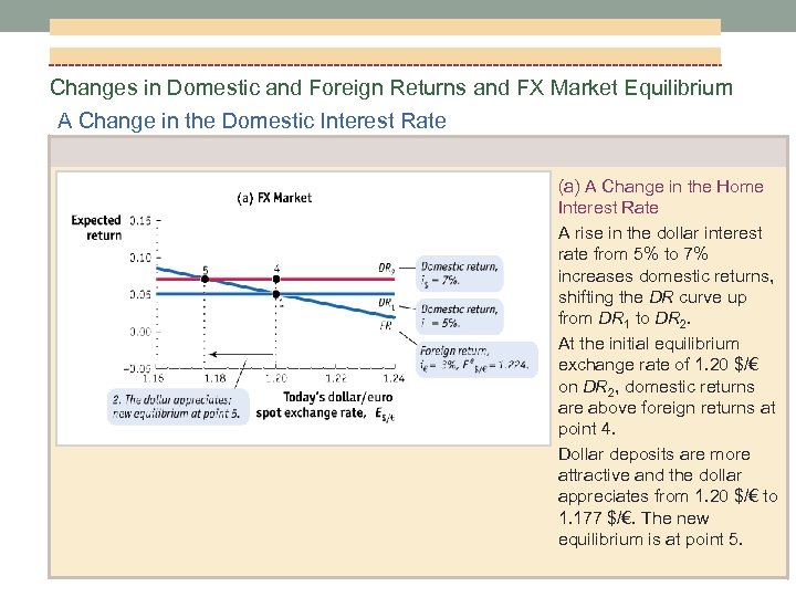Changes in Domestic and Foreign Returns and FX Market Equilibrium A Change in the Domestic Interest Rate (a) A Change in the Home Interest Rate A rise in the dollar interest rate from 5% to 7% increases domestic returns, shifting the DR curve up from DR 1 to DR 2. At the initial equilibrium exchange rate of 1. 20 $/€ on DR 2, domestic returns are above foreign returns at point 4. Dollar deposits are more attractive and the dollar appreciates from 1. 20 $/€ to 1. 177 $/€. The new equilibrium is at point 5.

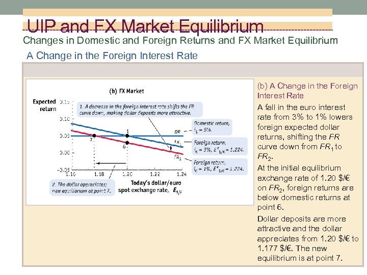UIP and FX Market Equilibrium Changes in Domestic and Foreign Returns and FX Market Equilibrium A Change in the Foreign Interest Rate (b) A Change in the Foreign Interest Rate A fall in the euro interest rate from 3% to 1% lowers foreign expected dollar returns, shifting the FR curve down from FR 1 to FR 2. At the initial equilibrium exchange rate of 1. 20 $/€ on FR 2, foreign returns are below domestic returns at point 6. Dollar deposits are more attractive and the dollar appreciates from 1. 20 $/€ to 1. 177 $/€. The new equilibrium is at point 7.

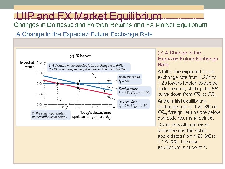UIP and FX Market Equilibrium Changes in Domestic and Foreign Returns and FX Market Equilibrium A Change in the Expected Future Exchange Rate (c) A Change in the Expected Future Exchange Rate A fall in the expected future exchange rate from 1. 224 to 1. 20 lowers foreign expected dollar returns, shifting the FR curve down from FR 1 to FR 2. At the initial equilibrium exchange rate of 1. 20 $/€ on FR 2, foreign returns are below domestic returns at point 6. Dollar deposits are more attractive and the dollar appreciates from 1. 20 $/€ to 1. 177 $/€. The new equilibrium is at point 7.

Interest Rates in the Short Run: Money Market Equilibrium in the Short Run: How Nominal Interest Rates Are Determined The Assumptions We make short-run assumptions that are quite different from the long-run assumptions of the PPP approach: — ■ In the short run, the price level is sticky; it is a known predetermined variable, fixed at P = P (the bar indicates a fixed value). ■ In the short run, the nominal interest rate i is fully flexible and adjusts to bring the money market to equilibrium. • The assumption of sticky prices, also called nominal rigidity, is common to the study of macroeconomics in the short run.

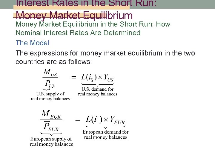Interest Rates in the Short Run: Money Market Equilibrium in the Short Run: How Nominal Interest Rates Are Determined The Model The expressions for money market equilibrium in the two countries are as follows:

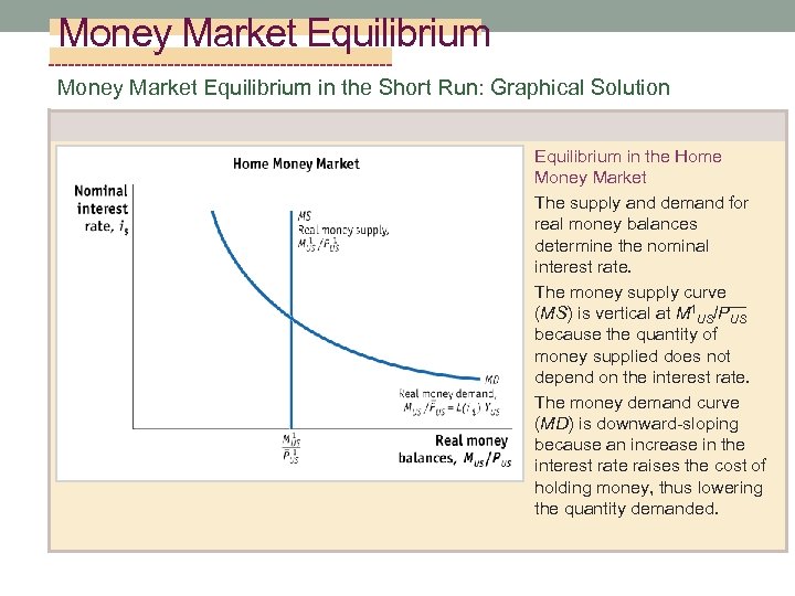Money Market Equilibrium in the Short Run: Graphical Solution Equilibrium in the Home Money Market The supply and demand for real money balances determine the nominal interest rate. The money supply curve (MS) is vertical at M 1 US/P— US because the quantity of money supplied does not depend on the interest rate. The money demand curve (MD) is downward-sloping because an increase in the interest rate raises the cost of holding money, thus lowering the quantity demanded.

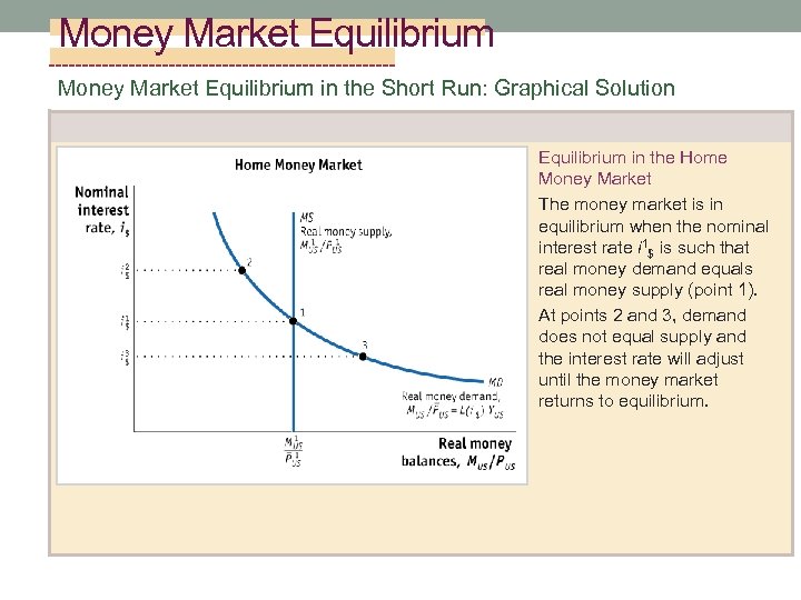Money Market Equilibrium in the Short Run: Graphical Solution Equilibrium in the Home Money Market The money market is in equilibrium when the nominal interest rate i 1$ is such that real money demand equals real money supply (point 1). At points 2 and 3, demand does not equal supply and the interest rate will adjust until the money market returns to equilibrium.

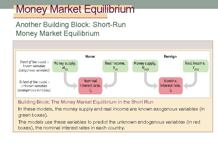Money Market Equilibrium Another Building Block: Short-Run Money Market Equilibrium Building Block: The Money Market Equilibrium in the Short Run In these models, the money supply and real income are known exogenous variables (in green boxes). The models use these variables to predict the unknown endogenous variables (in red boxes), the nominal interest rates in each country.

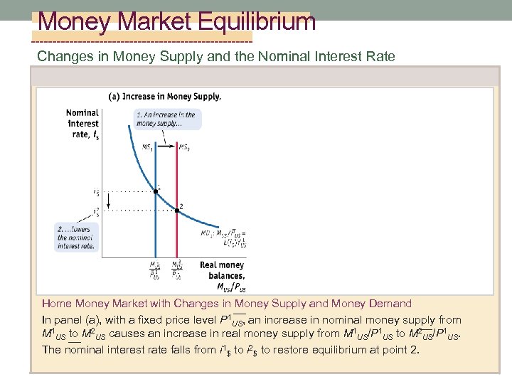Money Market Equilibrium Changes in Money Supply and the Nominal Interest Rate Home Money Market with Changes in Money Supply and Money Demand — In panel (a), with a fixed price level P 1 US, an increase in nominal money supply from — M 1 US to M 2 US causes an increase in real money supply from M 1 US/P 1 US to M 2 US/P 1 US. — The nominal interest rate falls from i 1$ to i 2$ to restore equilibrium at point 2.

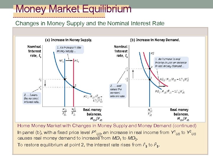Money Market Equilibrium Changes in Money Supply and the Nominal Interest Rate Home Money Market with Changes in Money Supply and Money Demand (continued) In panel (b), with a fixed price level P 1 US, an increase in real income from Y 1 US to Y 2 US — causes real money demand to increase from MD 1 to MD 2. To restore equilibrium at point 2, the interest rate rises from i 1$ to i 2$.

APPLICATION Can Central Banks Always Control the Interest Rate? A Lesson from the Crisis of 2008– 2009 • In the United States, the Federal Reserve sets as its policy rate the interest rate that it charges banks for overnight loans. • In normal times, changes in this cost of short-term funds for the banks are usually passed through into the market rates the banks charge to borrowers as well as on interbank loans between the banks themselves. • This process is one of the most basic elements in the so -called transmission mechanism through which the effects of monetary policy are eventually felt in the real economy.

APPLICATION Can Central Banks Always Control the Interest Rate? A Lesson from the Crisis of 2008– 2009 • In the recent crisis, although the Fed brought its policy rate all the way down from 5. 25% to 0% in 2007 and 2008, there was no similar decrease in market rates. • A second problem arose once policy rates hit the zero lower bound (ZLB). At that point, the central banks’ capacity to lower interest rate further was exhausted. However, many central banks wanted to keep applying downward pressure to market rates to calm financial markets. The Fed’s response was a policy of quantitative easing.

APPLICATION Can Central Banks Always Control the Interest Rate? A Lesson from the Crisis of 2008– 2009 The Fed engaged in a number of extraordinary policy actions to push more money out more quickly: 1. It expanded the range of credit securities it would accept as collateral to include lower-grade, privatesector bonds. 2. It expanded the range of securities that it would buy outright to include private-sector credit instruments such as commercial papers and mortgage-backed securities. 3. It expanded the range of counterparties from which it would buy securities to include some nonbank institutions such as primary dealers and money market funds.

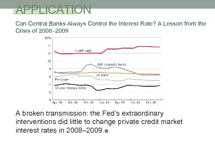APPLICATION Can Central Banks Always Control the Interest Rate? A Lesson from the Crisis of 2008– 2009 A broken transmission: the Fed’s extraordinary interventions did little to change private credit market interest rates in 2008– 2009. ■

Interest Rates in the Short Run: The Monetary Model: The Short Run versus the Long Run Consider the following example: the Home central bank that previously kept the money supply constant suddenly switches to an expansionary policy. In the following year, it allows the money supply to grow at a rate of 5%. ■ If such expansions are expected to be a permanent policy in the long run, the predictions of the long-run monetary approach and Fisher effect are clear. The Home interest rate rises in the long run. ■ If this expansion is expected to be temporary, then, all else equal, the immediate effect is an excess supply of real money balances. The home interest rate will then fall in the short run.

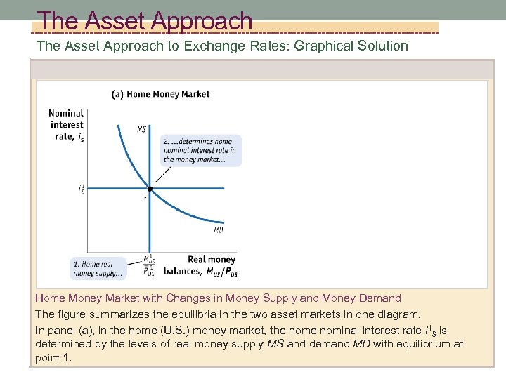The Asset Approach to Exchange Rates: Graphical Solution Home Money Market with Changes in Money Supply and Money Demand The figure summarizes the equilibria in the two asset markets in one diagram. In panel (a), in the home (U. S. ) money market, the home nominal interest rate i 1$ is determined by the levels of real money supply MS and demand MD with equilibrium at point 1.

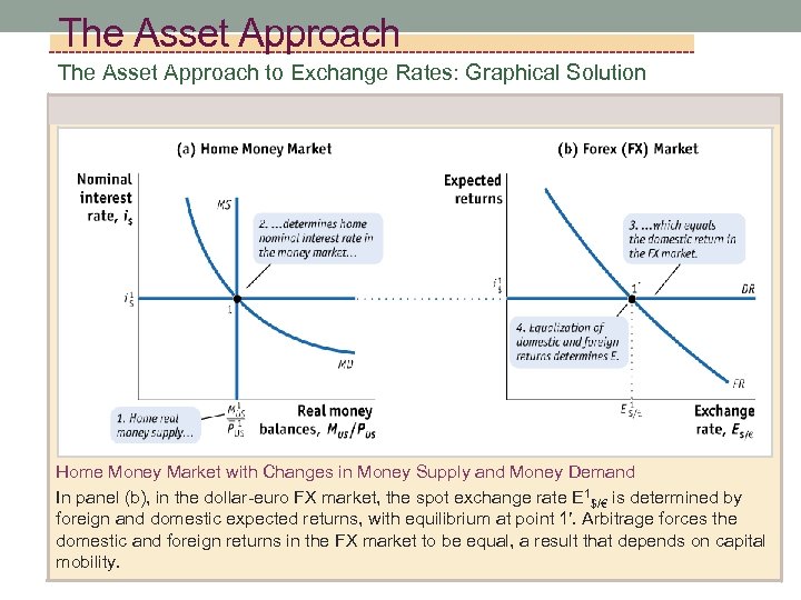The Asset Approach to Exchange Rates: Graphical Solution Home Money Market with Changes in Money Supply and Money Demand In panel (b), in the dollar-euro FX market, the spot exchange rate E 1$/€ is determined by foreign and domestic expected returns, with equilibrium at point 1′. Arbitrage forces the domestic and foreign returns in the FX market to be equal, a result that depends on capital mobility.

The Asset Approach Capital Mobility Is Crucial Our assumption that DR equals FR depends on capital mobility. If capital controls are imposed, there is no arbitrage and no reason why DR has to equal FR. Putting the Model to Work With this graphical apparatus in place, it is relatively straightforward to solve for the exchange rate given all the known (exogenous) variables we have specified previously.

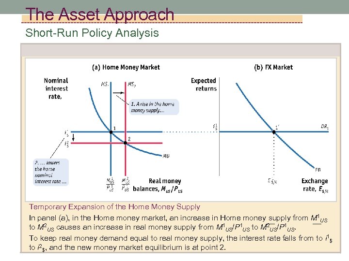The Asset Approach Short-Run Policy Analysis Temporary Expansion of the Home Money Supply In panel (a), in the Home money market, an increase in Home money supply from M 1 US — 2 to M 2 US causes an increase in real money supply from M 1 US/P 1 US to M— /P 1 US. US To keep real money demand equal to real money supply, the interest rate falls from to i 1$ to i 2$, and the new money market equilibrium is at point 2.

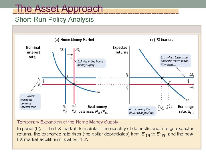The Asset Approach Short-Run Policy Analysis Temporary Expansion of the Home Money Supply In panel (b), in the FX market, to maintain the equality of domestic and foreign expected returns, the exchange rate rises (the dollar depreciates) from E 1$/€ to E 2$/€, and the new FX market equilibrium is at point 2′.

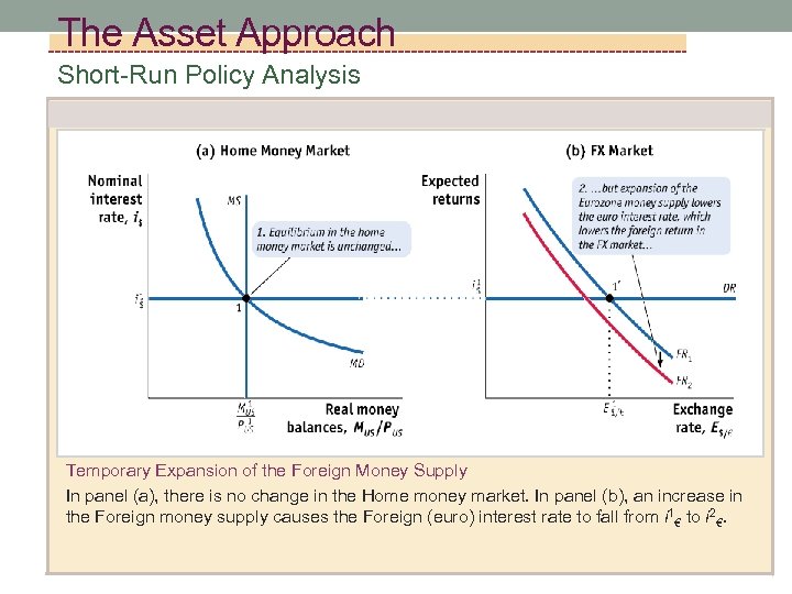The Asset Approach Short-Run Policy Analysis Temporary Expansion of the Foreign Money Supply In panel (a), there is no change in the Home money market. In panel (b), an increase in the Foreign money supply causes the Foreign (euro) interest rate to fall from i 1€ to i 2€.

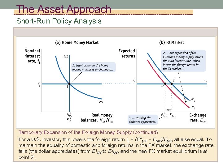The Asset Approach Short-Run Policy Analysis Temporary Expansion of the Foreign Money Supply (continued) For a U. S. investor, this lowers the foreign return i€ + (Ee$/ € − E$/€)/E$/€, all else equal. To maintain the equality of domestic and foreign returns in the FX market, the exchange rate falls (the dollar appreciates) from E 1$/€ to E 2$/€, and the new FX market equilibrium is at point 2′.

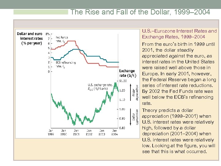The Rise and Fall of the Dollar, 1999– 2004 U. S. –Eurozone Interest Rates and Exchange Rates, 1999– 2004 From the euro’s birth in 1999 until 2001, the dollar steadily appreciated against the euro, as interest rates in the United States were raised well above those in Europe. In early 2001, however, the Federal Reserve began a long series of interest rate reductions. By 2002 the Fed Funds rate was well below the ECB’s refinancing rate. Theory predicts a dollar appreciation (1999– 2001) when U. S. interest rates were relatively high, followed by a dollar depreciation (2001– 2004) when U. S. interest rates were relatively low. Looking at the figure, you will see that this is what occurred.

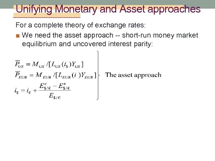Unifying Monetary and Asset approaches For a complete theory of exchange rates: ■ We need the asset approach -- short-run money market equilibrium and uncovered interest parity:

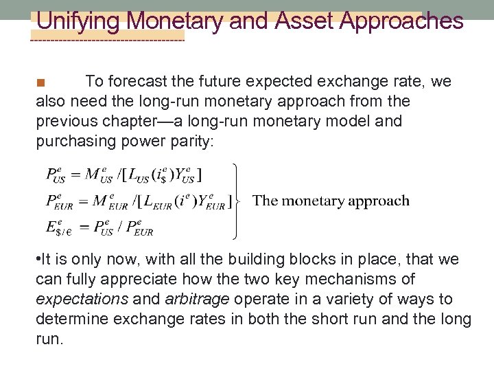Unifying Monetary and Asset Approaches ■ To forecast the future expected exchange rate, we also need the long-run monetary approach from the previous chapter—a long-run monetary model and purchasing power parity: • It is only now, with all the building blocks in place, that we can fully appreciate how the two key mechanisms of expectations and arbitrage operate in a variety of ways to determine exchange rates in both the short run and the long run.

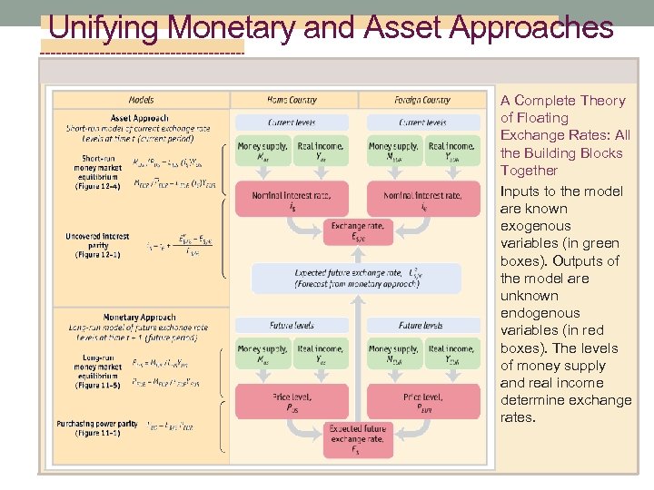Unifying Monetary and Asset Approaches A Complete Theory of Floating Exchange Rates: All the Building Blocks Together Inputs to the model are known exogenous variables (in green boxes). Outputs of the model are unknown endogenous variables (in red boxes). The levels of money supply and real income determine exchange rates.

Unifying Monetary and Asset Approaches Long-Run Policy Analysis Confessions of a Forex Trader In the world of exchange rate forecasting, three methodologies are generally used: 1. Economic fundamentals. 2. Politics 3. Technical methods A recent survey of U. K. forex traders provided some interesting insights into this world. One-third described their trading as “technically based, ” and one-third said their trades were “fundamentals-based”; others were jobbing or trading for clients.

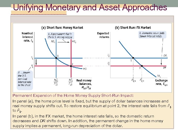Unifying Monetary and Asset Approaches Permanent Expansion of the Home Money Supply Short-Run Impact: In panel (a), the home price level is fixed, but the supply of dollar balances increases and real money supply shifts out. To restore equilibrium at point 2, the interest rate falls from i 1$ to i 2$. In panel (b), in the FX market, the home interest rate falls, so the domestic return decreases and DR shifts down. In addition, the permanent change in the home money supply implies a permanent, long-run depreciation of the dollar.

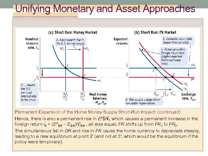Unifying Monetary and Asset Approaches Permanent Expansion of the Home Money Supply Short-Run Impact: (continued) Hence, there is also a permanent rise in Ee$/€, which causes a permanent increase in the foreign return i€ + (Ee$/€ − E$/€)/E$/€ , all else equal; FR shifts up from FR 1 to FR 2. The simultaneous fall in DR and rise in FR cause the home currency to depreciate steeply, leading to a new equilibrium at point 2′ (and not at 3′, which would be the equilibrium if the policy were temporary).

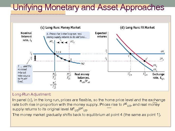Unifying Monetary and Asset Approaches Long-Run Adjustment: In panel (c), in the long run, prices are flexible, so the home price level and the exchange — rate both rise in proportion with the money supply. Prices rise to P 2 US, and real money — supply returns to its original level M 1 US/P 1 US. The money market gradually shifts back to equilibrium at point 4 (the same as point 1).

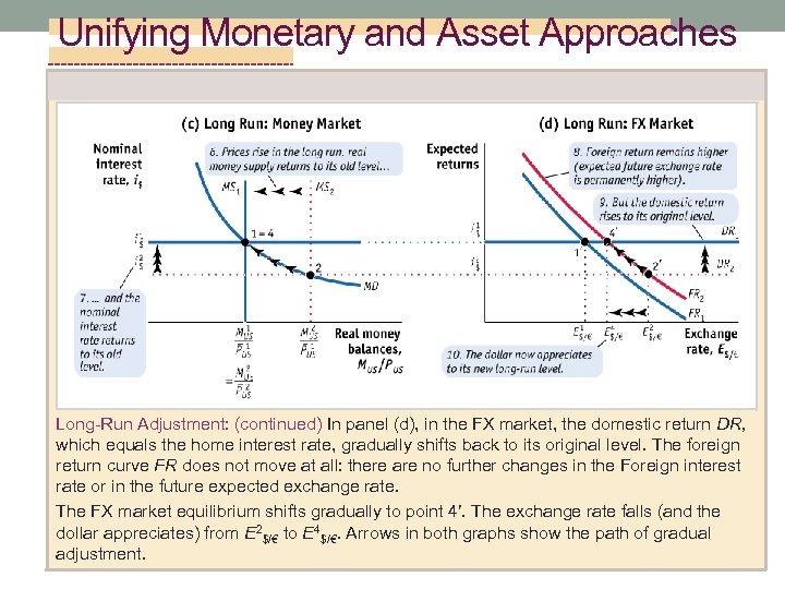Unifying Monetary and Asset Approaches Long-Run Adjustment: (continued) In panel (d), in the FX market, the domestic return DR, which equals the home interest rate, gradually shifts back to its original level. The foreign return curve FR does not move at all: there are no further changes in the Foreign interest rate or in the future expected exchange rate. The FX market equilibrium shifts gradually to point 4′. The exchange rate falls (and the dollar appreciates) from E 2$/€ to E 4$/€. Arrows in both graphs show the path of gradual adjustment.

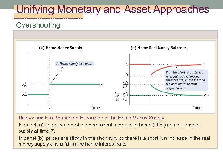Unifying Monetary and Asset Approaches Overshooting Responses to a Permanent Expansion of the Home Money Supply In panel (a), there is a one-time permanent increase in home (U. S. ) nominal money supply at time T. In panel (b), prices are sticky in the short run, so there is a short-run increase in the real money supply and a fall in the home interest rate.

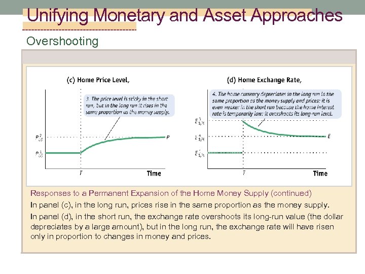Unifying Monetary and Asset Approaches Overshooting Responses to a Permanent Expansion of the Home Money Supply (continued) In panel (c), in the long run, prices rise in the same proportion as the money supply. In panel (d), in the short run, the exchange rate overshoots its long-run value (the dollar depreciates by a large amount), but in the long run, the exchange rate will have risen only in proportion to changes in money and prices.

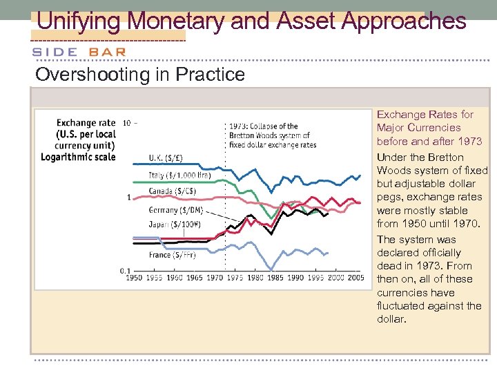Unifying Monetary and Asset Approaches Overshooting in Practice Exchange Rates for Major Currencies before and after 1973 Under the Bretton Woods system of fixed but adjustable dollar pegs, exchange rates were mostly stable from 1950 until 1970. The system was declared officially dead in 1973. From then on, all of these currencies have fluctuated against the dollar.

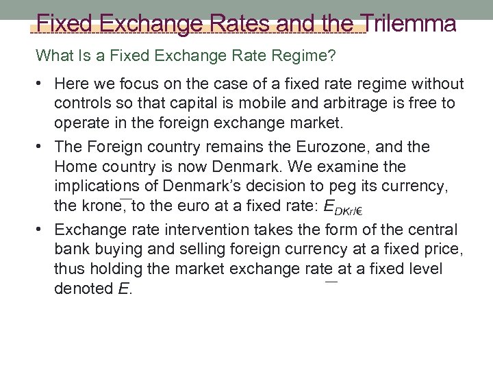Fixed Exchange Rates and the Trilemma What Is a Fixed Exchange Rate Regime? • Here we focus on the case of a fixed rate regime without controls so that capital is mobile and arbitrage is free to operate in the foreign exchange market. • The Foreign country remains the Eurozone, and the Home country is now Denmark. We examine the implications of Denmark’s decision to peg its currency, — the krone, to the euro at a fixed rate: EDKr/€ • Exchange rate intervention takes the form of the central bank buying and selling foreign currency at a fixed price, thus holding the market exchange rate at a fixed level — denoted E.

Fixed Exchange Rates and the Trilemma What Is a Fixed Exchange Rate Regime? • In the long run, fixing the exchange rate is one kind of nominal anchor. • Yet even if it allowed the krone to float but had some nominal anchor, Denmark’s monetary policy would still be constrained in the long run by the need to achieve its chosen nominal target. • What we now show is that a country with a fixed exchange rate faces monetary policy constraints not just in the long run but also in the short run.

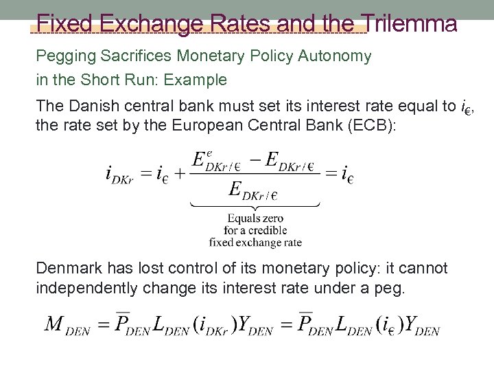Fixed Exchange Rates and the Trilemma Pegging Sacrifices Monetary Policy Autonomy in the Short Run: Example The Danish central bank must set its interest rate equal to i€, the rate set by the European Central Bank (ECB): Denmark has lost control of its monetary policy: it cannot independently change its interest rate under a peg.

Fixed Exchange Rates and the Trilemma Pegging Sacrifices Monetary Policy Autonomy in the Short Run: Example Our short-run theory still applies, but with a different chain of causality: ■ Under flexible exchange rates, the monetary authorities pick the money supply M. In the short run, the choice of M determines the interest rate i in the money market; in turn, via UIP, the level of i determines the exchange rate E. ■ The money supply is an input in the model (an exogenous variable), and the exchange rate is an output of the model (an endogenous variable).

Fixed Exchange Rates and the Trilemma Pegging Sacrifices Monetary Policy Autonomy in the Short Run: Example Our short-run theory still applies, but with a different chain of causality: ■ Under a fix, this logic is reversed. Home monetary authorities pick the fixed level of the exchange rate E. In the short run, a fixed E pins down the home interest rate i via UIP (forcing i to equal the foreign interest rate i*); ■ The level of i determines the level of the money supply M necessary to meet money demand. ■ The exchange rate is an input in the model (an exogenous variable), and the money supply is an output of the model (an endogenous variable).

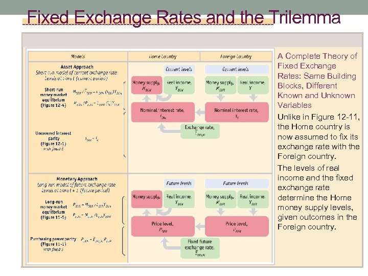Fixed Exchange Rates and the Trilemma A Complete Theory of Fixed Exchange Rates: Same Building Blocks, Different Known and Unknown Variables Unlike in Figure 12 -11, the Home country is now assumed to fix its exchange rate with the Foreign country. The levels of real income and the fixed exchange rate determine the Home money supply levels, given outcomes in the Foreign country.

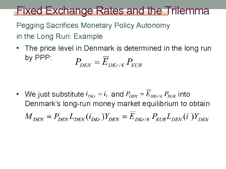Fixed Exchange Rates and the Trilemma Pegging Sacrifices Monetary Policy Autonomy in the Long Run: Example • The price level in Denmark is determined in the long run by PPP: • We just substitute and into Denmark’s long-run money market equilibrium to obtain

Fixed Exchange Rates and the Trilemma Pegging Sacrifices Monetary Policy Autonomy in the Long Run: Example Our long-run theory still applies, but with a different chain of causality: ■ Under a float, the home monetary authorities pick the money supply M. ■ The growth rate of M determines the interest rate i via the Fisher effect and also the price level P; in turn, via PPP, the level of P determines the exchange rate E. ■ The money supply is an input in the model (an exogenous variable), and the exchange rate is an output of the model (an endogenous variable).

Fixed Exchange Rates and the Trilemma Pegging Sacrifices Monetary Policy Autonomy in the Long Run: Example Our long-run theory still applies, but with a different chain of causality: ■ Under monetary authorities pick the exchange rate E. ■ Under In the long run, the choice of E determines the price level P via PPP, and also the interest rate i via UIP; ■ These, in turn, determine the necessary level of the money supply M. ■ The exchange rate is an input in the model (an exogenous variable), and the money supply is an output of the model (an endogenous variable).

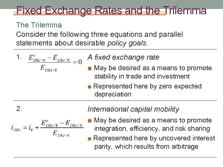Fixed Exchange Rates and the Trilemma The Trilemma Consider the following three equations and parallel statements about desirable policy goals. 1. A fixed exchange rate ■ May be desired as a means to promote stability in trade and investment ■ Represented here by zero expected depreciation 2. International capital mobility ■ May be desired as a means to promote integration, efficiency, and risk sharing ■ Represented here by uncovered interest parity, which results from arbitrage

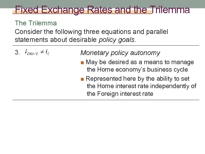Fixed Exchange Rates and the Trilemma The Trilemma Consider the following three equations and parallel statements about desirable policy goals. 3. Monetary policy autonomy ■ May be desired as a means to manage the Home economy’s business cycle ■ Represented here by the ability to set the Home interest rate independently of the Foreign interest rate

Fixed Exchange Rates and the Trilemma The Trilemma • 1, 2, and 3 show that : ■ 1 and 2 imply not 3 (1 and 2 imply interest equality, contradicting 3). ■ 2 and 3 imply not 1 (2 and 3 imply an expected change in E, contradicting 1). ■ 3 and 1 imply not 2 (3 and 1 imply a difference between domestic and foreign returns, contradicting 2). • This result, known as the trilemma, is one of the most important ideas in international macroeconomics.

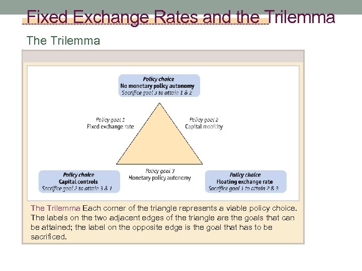Fixed Exchange Rates and the Trilemma The Trilemma Each corner of the triangle represents a viable policy choice. The labels on the two adjacent edges of the triangle are the goals that can be attained; the label on the opposite edge is the goal that has to be sacrificed.

Fixed Exchange Rates and the Trilemma The Trilemma Intermediate Regimes • The lessons of the trilemma most clearly apply when the policies are at the ends of a spectrum: a hard peg or a float, perfect capital mobility or immobility, complete autonomy or none at all. • But sometimes a country may not be fully in one of the three corners: the rigidity of the peg, the degree of capital mobility, and the independence of monetary policy could be partial rather than full.

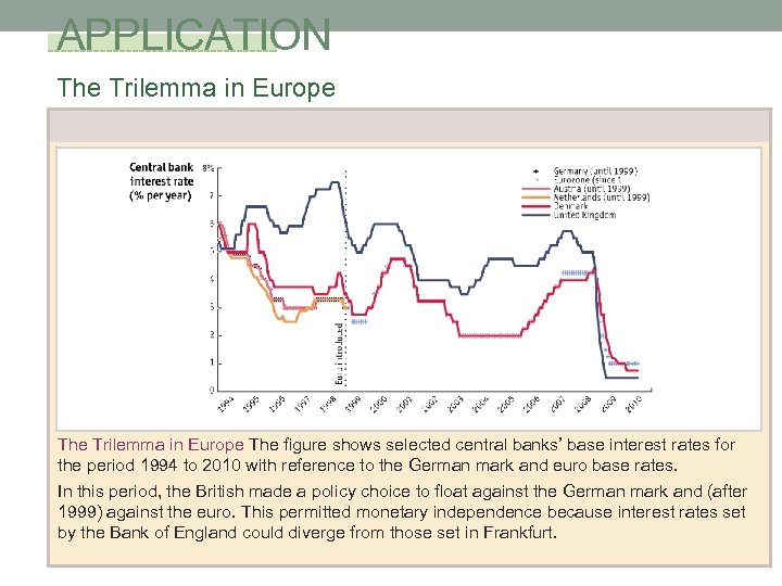APPLICATION The Trilemma in Europe The figure shows selected central banks’ base interest rates for the period 1994 to 2010 with reference to the German mark and euro base rates. In this period, the British made a policy choice to float against the German mark and (after 1999) against the euro. This permitted monetary independence because interest rates set by the Bank of England could diverge from those set in Frankfurt.

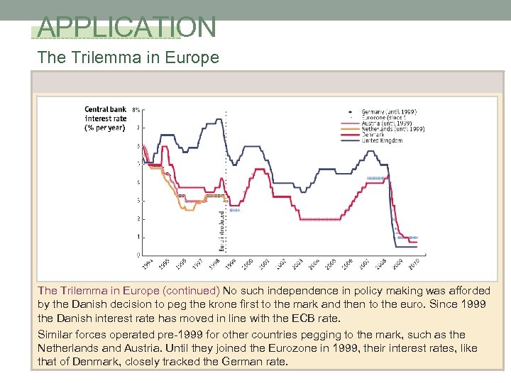APPLICATION The Trilemma in Europe (continued) No such independence in policy making was afforded by the Danish decision to peg the krone first to the mark and then to the euro. Since 1999 the Danish interest rate has moved in line with the ECB rate. Similar forces operated pre-1999 for other countries pegging to the mark, such as the Netherlands and Austria. Until they joined the Eurozone in 1999, their interest rates, like that of Denmark, closely tracked the German rate.