Lecture VI Adaptive Systems Zhixin Liu Complex Systems

Lecture VI: Adaptive Systems Zhixin Liu Complex Systems Research Center, Academy of Mathematics and Systems Sciences, CAS

In the last lecture, we talked about Game Theory An embodiment of the complex interactions among individuals l Nash equilibrium l Evolutionarily stable strategy

In this lecture, we will talk about Adaptive Systems

Adaptation To adapt: to change oneself to conform to a new or changed circumstance. Ø What we know from the new circumstance? Adaptive estimation, learning, identification Ø How to do the corresponding response? Control/decision making

Why Adaptation? Uncertainties always exist in modeling of practical systems. Adaptation can reduce the uncertainties by using the system information. Adaptation is an important embodiment of human intelligence.

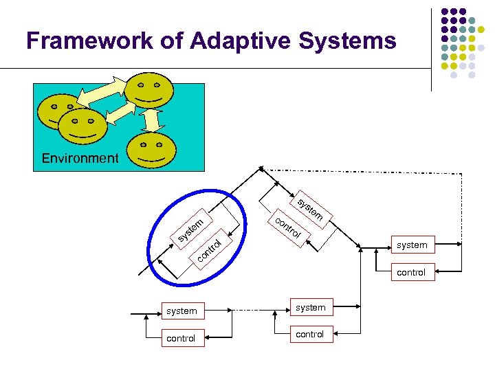Framework of Adaptive Systems Environment co nt sy ste m m te ro s sy l tro on l system c control system control

Two levels of adaptation l Individual: learn and adapt l Population level Ø Ø Ø Death of old individuals Creation of new individuals Hierarchy

Some Examples Adaptive control systems adaptation in a single agent Iterated prisoner’s dilemma adaptation among agents

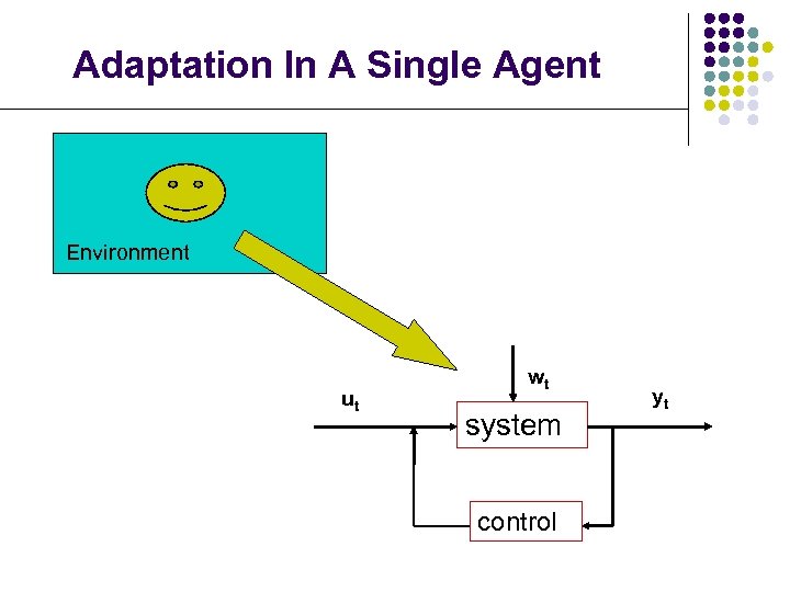Adaptation In A Single Agent Environment ut wt system control yt

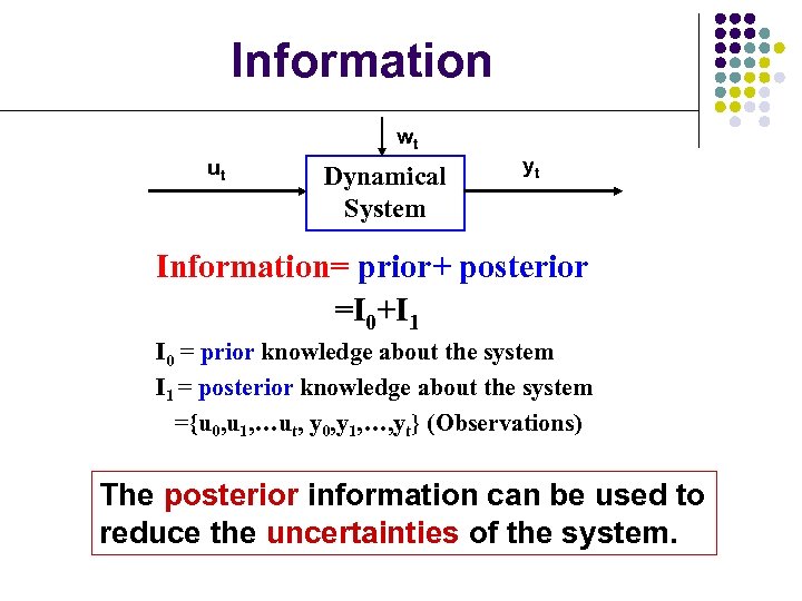Information wt ut Dynamical System yt Information= prior+ posterior =I 0+I 1 I 0 = prior knowledge about the system I 1 = posterior knowledge about the system ={u 0, u 1, …ut, y 0, y 1, …, yt} (Observations) The posterior information can be used to reduce the uncertainties of the system.

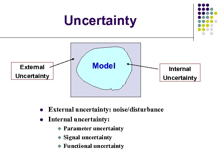Uncertainty Model External Uncertainty l l Internal Uncertainty External uncertainty: noise/disturbance Internal uncertainty: u u u Parameter uncertainty Signal uncertainty Functional uncertainty

Adaptation To adapt: to change oneself to conform to a new or changed circumstance. Ø What we know from the new circumstance? Adaptive estimation, learning, identification Ø How to do the corresponding response? Control/decision making

Adaptive Estimation

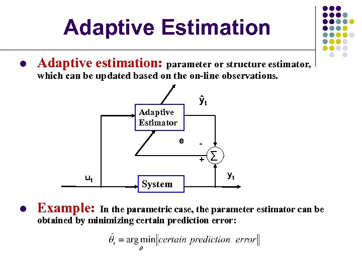Adaptive Estimation l Adaptive estimation: parameter or structure estimator, which can be updated based on the on-line observations. ŷt Adaptive Estimator e + ∑ ut l Example: System yt In the parametric case, the parameter estimator can be obtained by minimizing certain prediction error:

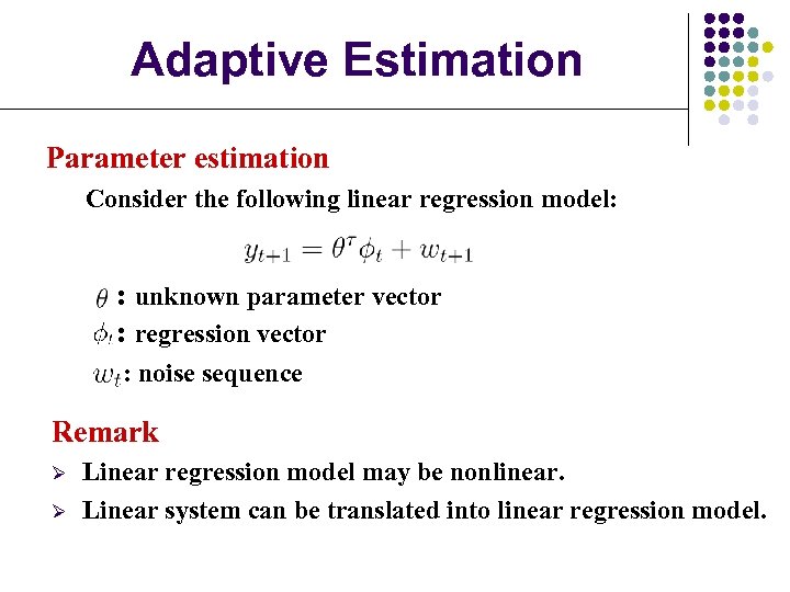Adaptive Estimation Parameter estimation Consider the following linear regression model: : unknown parameter vector : regression vector : noise sequence Remark Ø Ø Linear regression model may be nonlinear. Linear system can be translated into linear regression model.

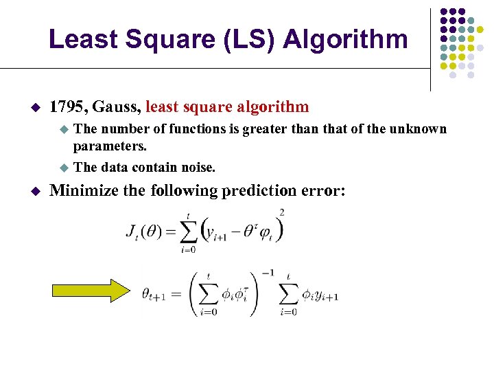Least Square (LS) Algorithm u 1795, Gauss, least square algorithm The number of functions is greater than that of the unknown parameters. u The data contain noise. u u Minimize the following prediction error:

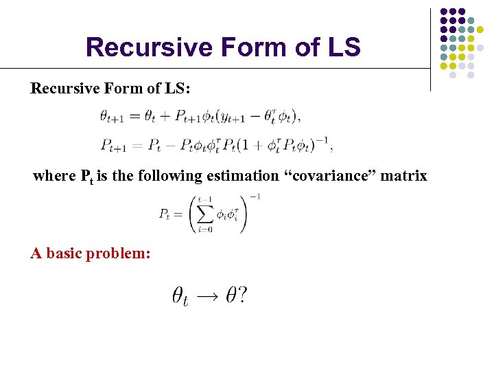Recursive Form of LS: where Pt is the following estimation “covariance” matrix A basic problem:

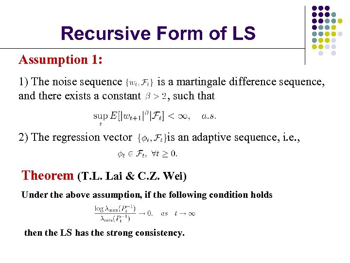Recursive Form of LS Assumption 1: 1) The noise sequence and there exists a constant 2) The regression vector is a martingale difference sequence, , such that is an adaptive sequence, i. e. , Theorem (T. L. Lai & C. Z. Wei) Under the above assumption, if the following condition holds then the LS has the strong consistency.

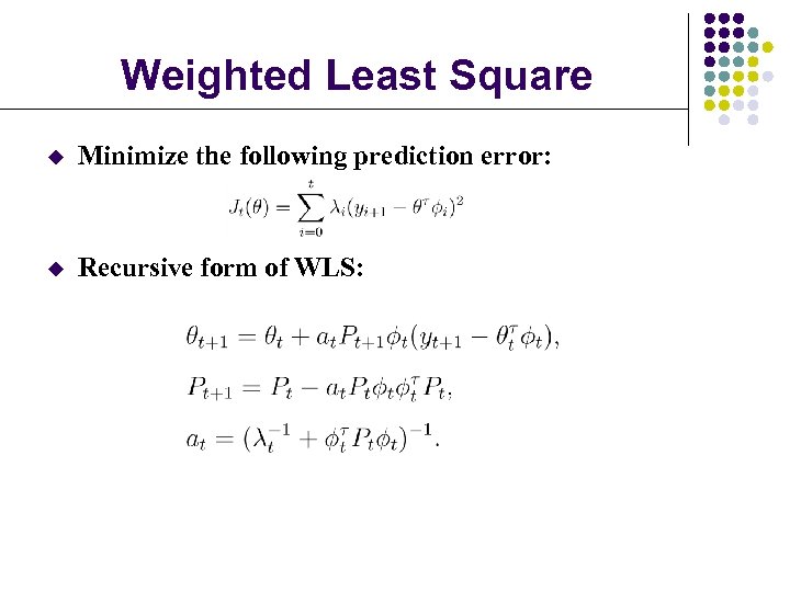Weighted Least Square u Minimize the following prediction error: u Recursive form of WLS:

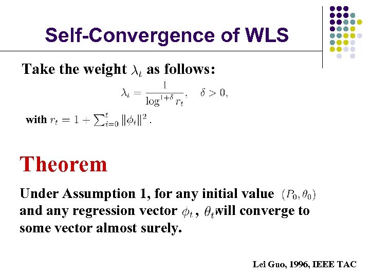Self-Convergence of WLS Take the weight with as follows: . Theorem Under Assumption 1, for any initial value and any regression vector , will converge to some vector almost surely. Lei Guo, 1996, IEEE TAC

Adaptation To adapt: to change oneself to conform to a new or changed circumstance. Ø What we know from the new circumstance? Adaptive estimation, learning, identification Ø How to do the corresponding response? Control/decision making

Adaptive Control

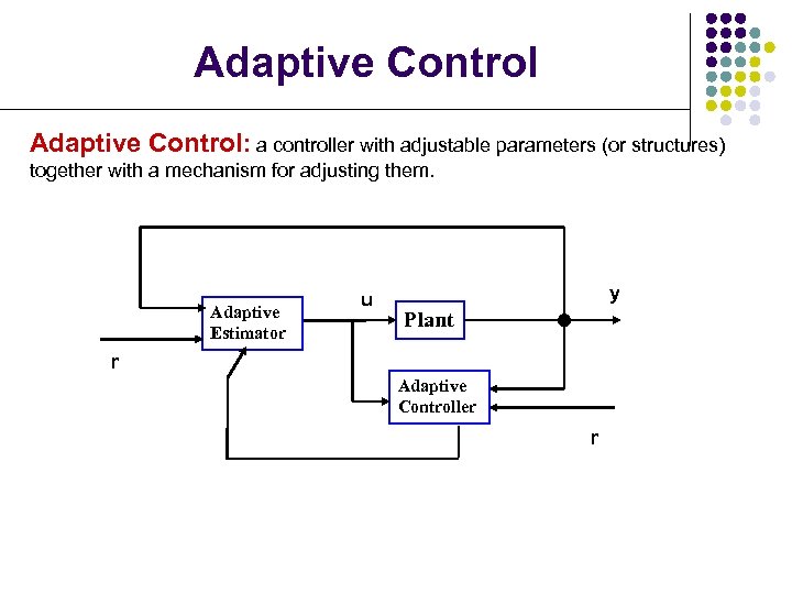Adaptive Control: a controller with adjustable parameters (or structures) together with a mechanism for adjusting them. Adaptive Estimator u y Plant r Adaptive Controller r

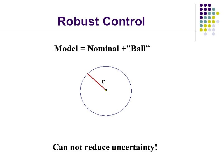Robust Control Model = Nominal +”Ball” r Can not reduce uncertainty!

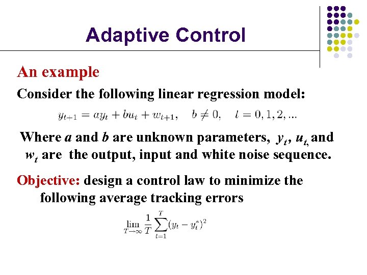Adaptive Control An example Consider the following linear regression model: Where a and b are unknown parameters, yt , ut, and wt are the output, input and white noise sequence. Objective: design a control law to minimize the following average tracking errors

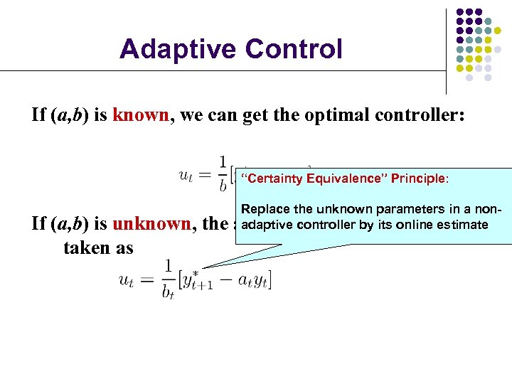Adaptive Control If (a, b) is known, we can get the optimal controller: “Certainty Equivalence” Principle: If (a, b) is unknown, the taken as Replace the unknown parameters in a nonadaptive controller by its can estimate adaptive controller online be

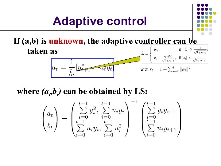Adaptive control If (a, b) is unknown, the adaptive controller can be taken as with where (at, bt) can be obtained by LS:

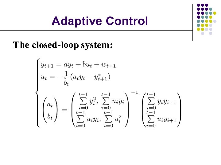Adaptive Control The closed-loop system:

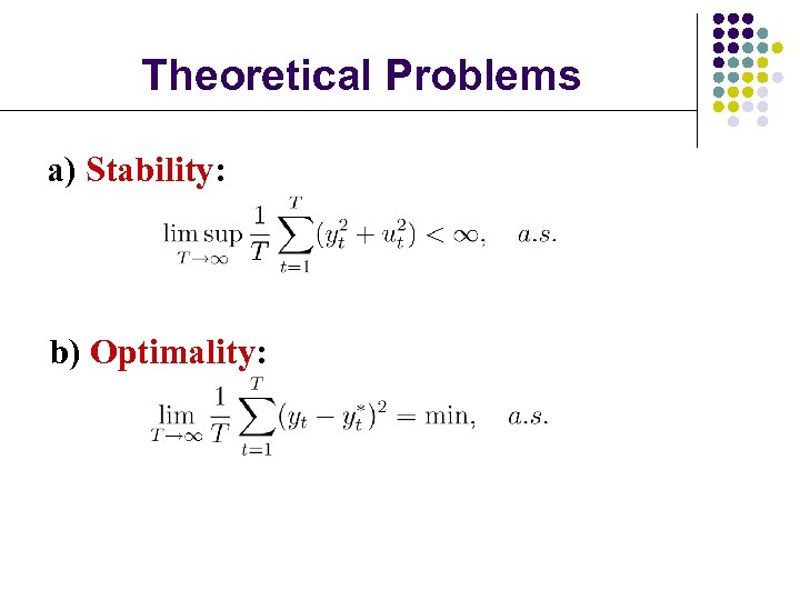Theoretical Problems a) Stability: b) Optimality:

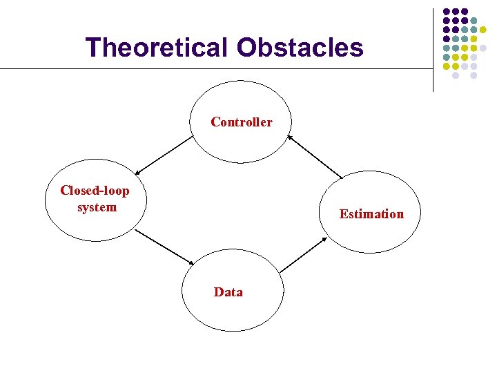Theoretical Obstacles Controller Closed-loop system Estimation Data

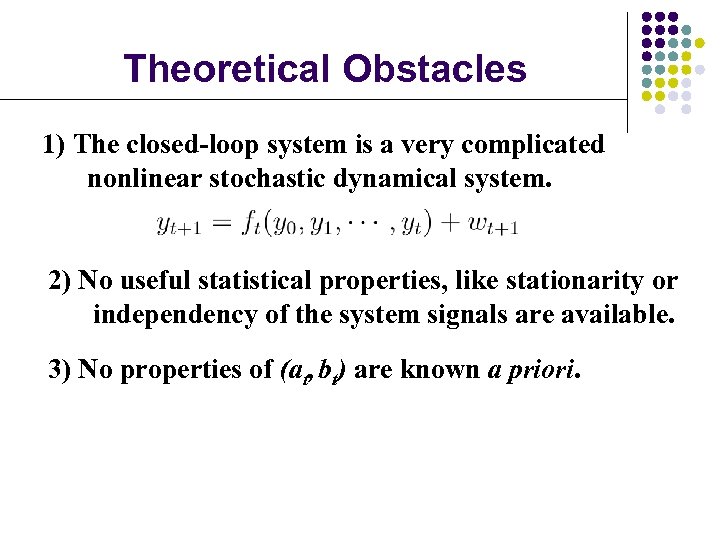Theoretical Obstacles 1) The closed-loop system is a very complicated nonlinear stochastic dynamical system. 2) No useful statistical properties, like stationarity or independency of the system signals are available. 3) No properties of (at, bt) are known a priori.

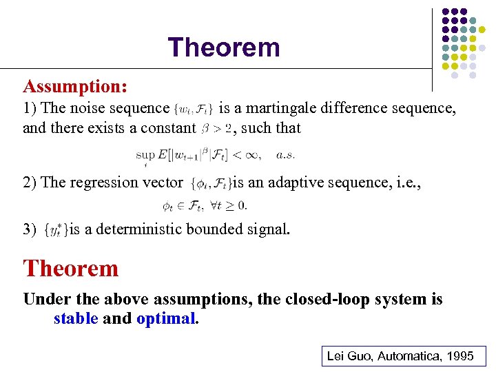Theorem Assumption: 1) The noise sequence and there exists a constant 2) The regression vector 3) is a martingale difference sequence, , such that is an adaptive sequence, i. e. , is a deterministic bounded signal. Theorem Under the above assumptions, the closed-loop system is stable and optimal. Lei Guo, Automatica, 1995

Some Examples Adaptive control systems adaptation in a single agent Iterated prisoner’s dilemma adaptation among agents

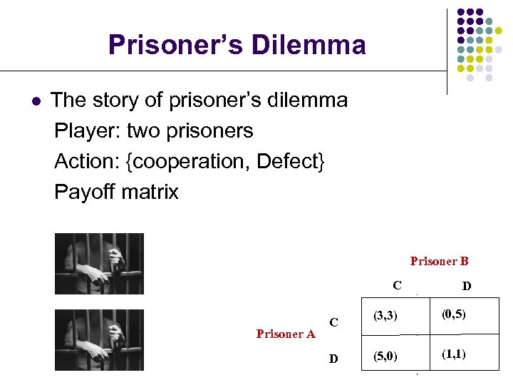Prisoner’s Dilemma l The story of prisoner’s dilemma Player: two prisoners Action: {cooperation, Defect} Payoff matrix Prisoner B C Prisoner A C D D (3, 3) (0, 5) (5, 0) (1, 1)

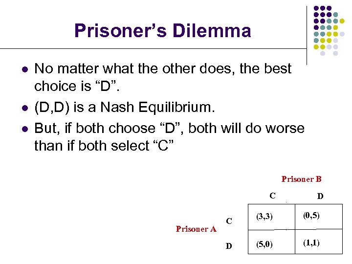Prisoner’s Dilemma l l l No matter what the other does, the best choice is “D”. (D, D) is a Nash Equilibrium. But, if both choose “D”, both will do worse than if both select “C” Prisoner B C Prisoner A C D D (3, 3) (0, 5) (5, 0) (1, 1)

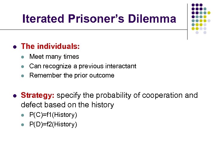Iterated Prisoner’s Dilemma l The individuals: l l Meet many times Can recognize a previous interactant Remember the prior outcome Strategy: specify the probability of cooperation and defect based on the history l l P(C)=f 1(History) P(D)=f 2(History)

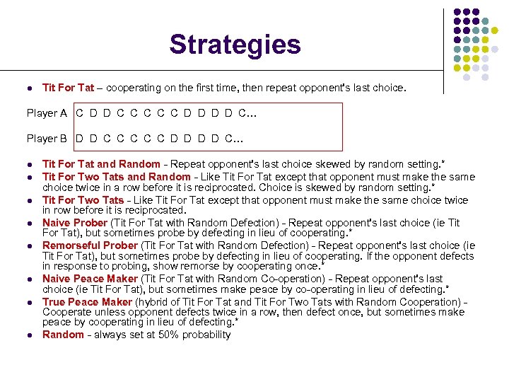
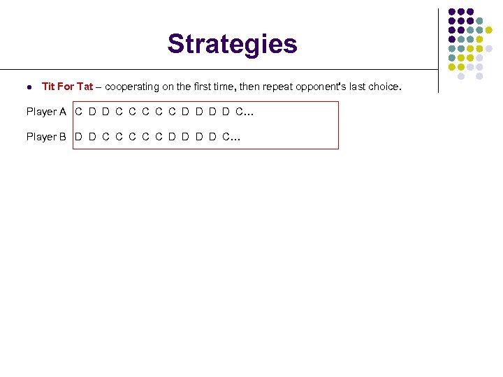Strategies l Tit For Tat – cooperating on the first time, then repeat opponent's last choice. Player A C D D C C C D D C… Player B D D C C C D D C… l l l l Tit For Tat and Random - Repeat opponent's last choice skewed by random setting. * Tit For Two Tats and Random - Like Tit For Tat except that opponent must make the same choice twice in a row before it is reciprocated. Choice is skewed by random setting. * Tit For Two Tats - Like Tit For Tat except that opponent must make the same choice twice in row before it is reciprocated. Naive Prober (Tit For Tat with Random Defection) - Repeat opponent's last choice (ie Tit For Tat), but sometimes probe by defecting in lieu of cooperating. * Remorseful Prober (Tit For Tat with Random Defection) - Repeat opponent's last choice (ie Tit For Tat), but sometimes probe by defecting in lieu of cooperating. If the opponent defects in response to probing, show remorse by cooperating once. * Naive Peace Maker (Tit For Tat with Random Co-operation) - Repeat opponent's last choice (ie Tit For Tat), but sometimes make peace by co-operating in lieu of defecting. * True Peace Maker (hybrid of Tit For Tat and Tit For Two Tats with Random Cooperation) Cooperate unless opponent defects twice in a row, then defect once, but sometimes make peace by cooperating in lieu of defecting. * Random - always set at 50% probability

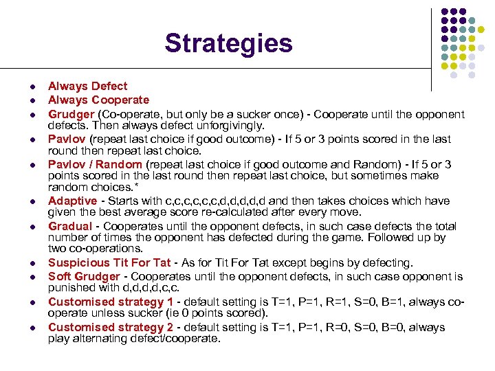Strategies l l l Always Defect Always Cooperate Grudger (Co-operate, but only be a sucker once) - Cooperate until the opponent defects. Then always defect unforgivingly. Pavlov (repeat last choice if good outcome) - If 5 or 3 points scored in the last round then repeat last choice. Pavlov / Random (repeat last choice if good outcome and Random) - If 5 or 3 points scored in the last round then repeat last choice, but sometimes make random choices. * Adaptive - Starts with c, c, c, d, d, d and then takes choices which have given the best average score re-calculated after every move. Gradual - Cooperates until the opponent defects, in such case defects the total number of times the opponent has defected during the game. Followed up by two co-operations. Suspicious Tit For Tat - As for Tit For Tat except begins by defecting. Soft Grudger - Cooperates until the opponent defects, in such case opponent is punished with d, d, c, c. Customised strategy 1 - default setting is T=1, P=1, R=1, S=0, B=1, always cooperate unless sucker (ie 0 points scored). Customised strategy 2 - default setting is T=1, P=1, R=0, S=0, B=0, always play alternating defect/cooperate.

Iterated Prisoner’s Dilemma l Which strategy can thrive/what is the good strategy? Robert Axelrod, 1980 s l A computer round-robin tournament l l l The first round The second round AXELROD R. 1987. The evolution of strategies in the iterated Prisoners' Dilemma. In L. Davis, editor, Genetic Algorithms and Simulated Annealing. Morgan Kaufmann, Los Altos, CA.

Characters of “good” strategies l Goodness: never defect first l l l Forgiveness: may revenge, but the memory is short. l l l First round: the first eight strategies with “goodness” Second round: fourteen strategies with “goodness” in the first fifteen strategies “Grudger” is not s strategy with “forgiveness” “Goodness” and “forgiveness” is a kind of collective behavior. For a single agent, defect is the best strategy.

Evolution of the Strategies l Evolve “good” strategies by genetic algorithm (GA)

Some Notations in GA l l l String: the individuals, and it is used to represent the chromosome in genetics. Population: the set of the individuals Population size: the number of the individuals Gene: the elements of the string E. g. , S＝ 1011, where 1，0，1，1 are called genes. Fitness: the adaptation of the agent for the circumstance From Jing Han’s PPT

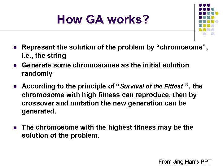How GA works? l l Represent the solution of the problem by “chromosome”, i. e. , the string Generate some chromosomes as the initial solution randomly l According to the principle of “Survival of the Fittest ”, the chromosome with high fitness can reproduce, then by crossover and mutation the new generation can be generated. l The chromosome with the highest fitness may be the solution of the problem. From Jing Han’s PPT

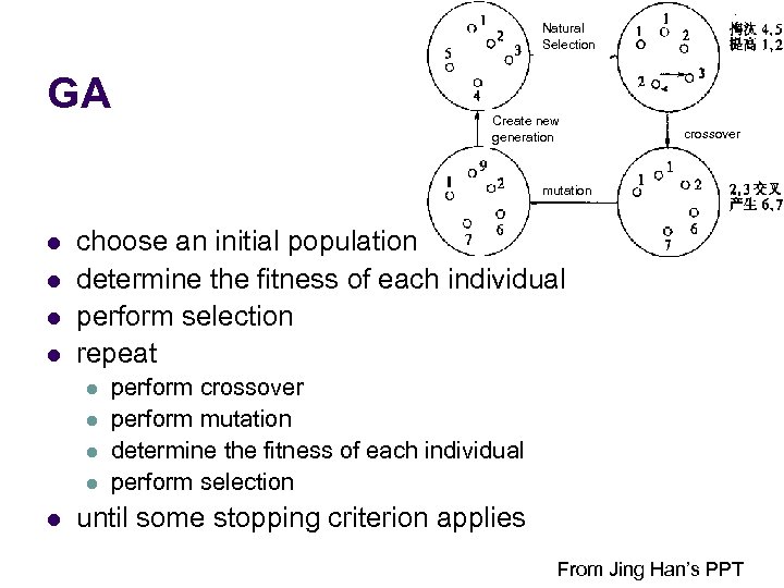Natural Selection GA Create new generation crossover mutation l l choose an initial population determine the fitness of each individual perform selection repeat l l l perform crossover perform mutation determine the fitness of each individual perform selection until some stopping criterion applies From Jing Han’s PPT

Some Remarks On GA l l The GA search the optimal solution from a set of solution, rather than a single solution The search space is large: {0, 1}L GA is a random algorithm, since selection, crossover and mutation are all random operations. Suitable for the following situation: l l l There is structure in the search space but it is not wellunderstood The inputs are non-stationary (i. e. , the environment is changing) The goal is not global optimization, but finding a reasonably good solution quickly

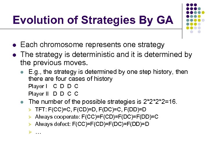Evolution of Strategies By GA l l Each chromosome represents one strategy The strategy is deterministic and it is determined by the previous moves. l E. g. , the strategy is determined by one step history, then there are four cases of history Player I C D D C Player II D D C C l The number of the possible strategies is 2*2*2*2=16. Ø TFT: F(CC)=C, F(CD)=D, F(DC)=C, F(DD)=D Always cooperate: F(CC)=F(CD)=F(DC)=F(DD)=C Always defect: F(CC)=F(CD)=F(DC)=F(DD)=D Ø … Ø Ø

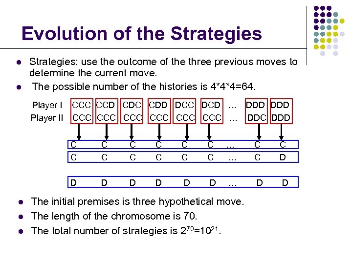Evolution of the Strategies l l Strategies: use the outcome of the three previous moves to determine the current move. The possible number of the histories is 4*4*4=64. Player II CCC CCD CDC CDD DCC DCD … DDD CCC CCC CCC … DDC DDD C C l l C C C C … … C C C D D l C C D D D … D D The initial premises is three hypothetical move. The length of the chromosome is 70. The total number of strategies is 270≈1021.

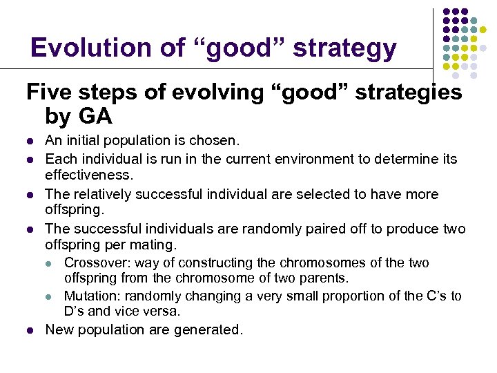Evolution of “good” strategy Five steps of evolving “good” strategies by GA l l l An initial population is chosen. Each individual is run in the current environment to determine its effectiveness. The relatively successful individual are selected to have more offspring. The successful individuals are randomly paired off to produce two offspring per mating. l Crossover: way of constructing the chromosomes of the two offspring from the chromosome of two parents. l Mutation: randomly changing a very small proportion of the C’s to D’s and vice versa. New population are generated.

Evolution of the Strategies Some parameters: l l l The population size in each generation is 20. Each game consists of 151 moves. Each of them meet eight representatives, and this made about 24, 000 moves per generation. A run consists of 50 generation Forty runs were conducted.

Results l l l The median member is as successful as TFT Most of the strategies is resemble TFT Some of them have the similar patterns as TFT l l l Do not rock the boat: continue to cooperate after the mutual cooperation Be provocable: defect when the other player defects out of the blue Accept an apology: continue to cooperate after cooperation has been restored Forget: cooperate when mutual cooperation has been restored after an exploitation Accept a rut: defect after three mutual defections

What is a “good” strategy? l l l TFT is a good strategy? Tit For Two Tats may be the best strategy in the first round, but it is not a good strategy in the second round. “Good” strategy depends on other strategies, i. e. , environment. Evolutionarily stable strategy

Evolutionarily stable strategy (ESS) l l Introduced by John Maynard Smith and George R. Price in 1973 ESS means evolutionarily stable strategy, that is “a strategy such that, if all member of the population adopt it, then no mutant strategy could invade the population under the influence of natural selection. ” John Maynard Smith, “Evolution and the Theory of Games” l ESS is robust for evolution, it can not be invaded by mutation.

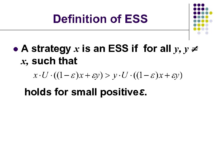Definition of ESS l A strategy x is an ESS if for all y, y x, such that holds for small positiveε.

ESS in IPD l l l Tit For Tat can not be invaded by the wiliness strategies, such as always defect. TFT can be invaded by “goodness” strategies, such as “always cooperate”, “Tit For Two Tats” and “Suspicious Tit For Tat ” Tit For Tat is not a strict ESS. “Always Cooperate” can be invaded by “Always Defect”. “Always Defect ” is an ESS.

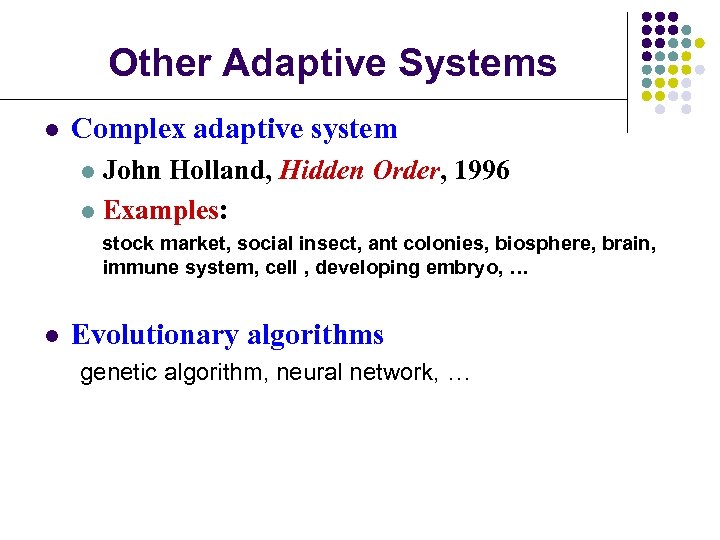Other Adaptive Systems l Complex adaptive system John Holland, Hidden Order, 1996 l Examples: l stock market, social insect, ant colonies, biosphere, brain, immune system, cell , developing embryo, … l Evolutionary algorithms genetic algorithm, neural network, …

References l Lei Guo, Self-convergence of weighted least-squares with applications to stochastic adaptive control, IEEE Trans. Automat. Contr. , 1996, 41(1): 79 -89. l Lei Guo, Convergence and logarithm laws of self-tuning regulators, 1995, Automatica, 31(3): 435 -450. l Lei Guo, Adaptive systems theory: some basic concepts, methods and results, Journal of Systems Science and Complexity, 16(3): 293 -306. l Drew Fudenberg, Jean Tirole, Game Theory, The MIT Press, 1991. l AXELROD R. 1987, The evolution of strategies in the iterated Prisoners' Dilemma. In L. Davis, editor, Genetic Algorithms and Simulated Annealing. Morgan Kaufmann, Los Altos, CA. l Richard Dawkins, The Selfish Gene, Oxford University Press. l John Holland, Hidden Order, 1996.

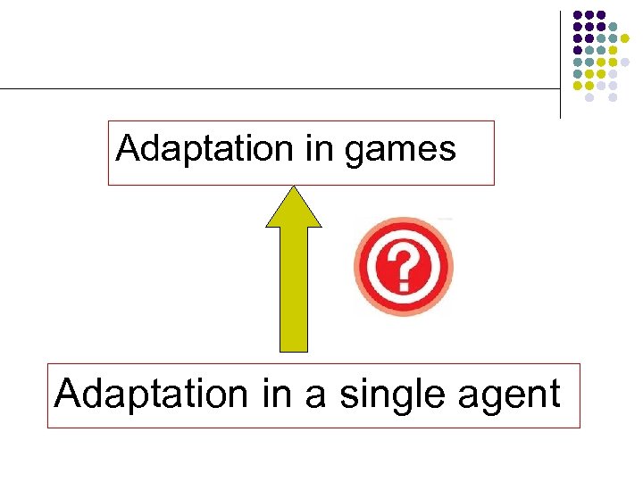Adaptation in games Adaptation in a single agent

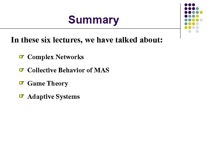Summary In these six lectures, we have talked about: Complex Networks Collective Behavior of MAS Game Theory Adaptive Systems

Summary In these six lectures, we have talked about: Complex Networks: Topology Collective Behavior of MAS Game Theory Adaptive Systems

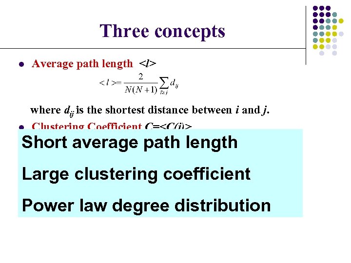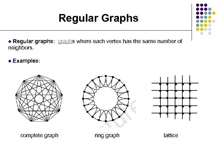Three concepts l Average path length l where dij is the shortest distance between i and j. Clustering Coefficient C= Short average path length Large distribution Degree clustering coefficient l P(k)=probability that the randomly chosen node i has Power neighbors exactly k law degree distribution

Regular Graphs Regular graphs: graphs where each vertex has the same number of neighbors. l l Examples: l l l l l ring graph l l complete graph l l lattice

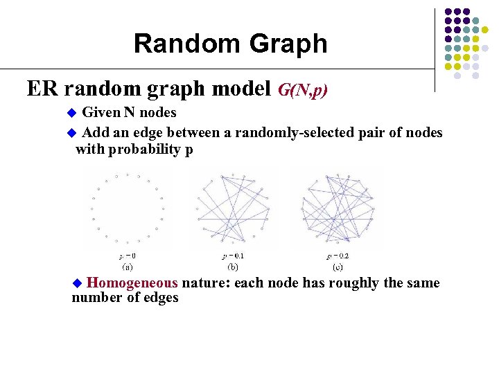Random Graph ER random graph model G(N, p) Given N nodes u Add an edge between a randomly-selected pair of nodes with probability p u Homogeneous nature: each node has roughly the same number of edges u

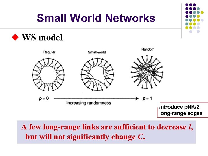Small World Networks u WS model Introduce p. NK/2 long-range edges A few long-range links are sufficient to decrease l, but will not significantly change C.

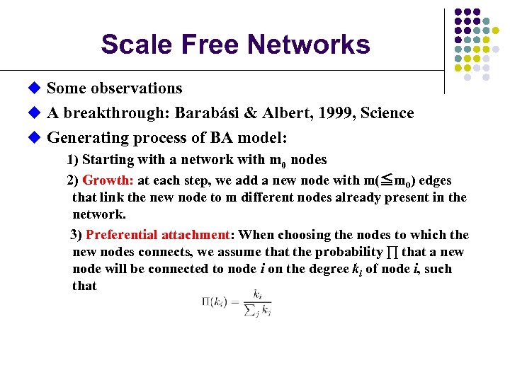Scale Free Networks u Some observations u A breakthrough: Barabási & Albert, 1999, Science u Generating process of BA model: 1) Starting with a network with m 0 nodes 2) Growth: at each step, we add a new node with m(≦m 0) edges that link the new node to m different nodes already present in the network. 3) Preferential attachment: When choosing the nodes to which the new nodes connects, we assume that the probability ∏ that a new node will be connected to node i on the degree ki of node i, such that

Summary In these six lectures, we have talked about: Complex Networks: Topology Collective Behavior of MAS: More is different Game Theory Adaptive Systems

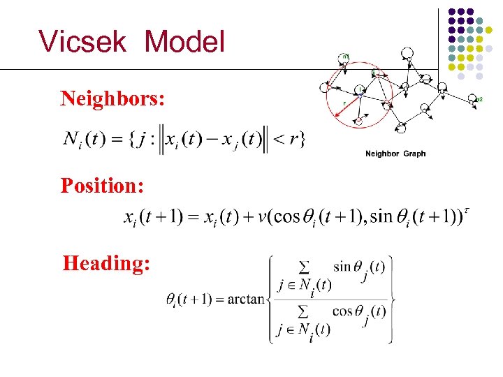
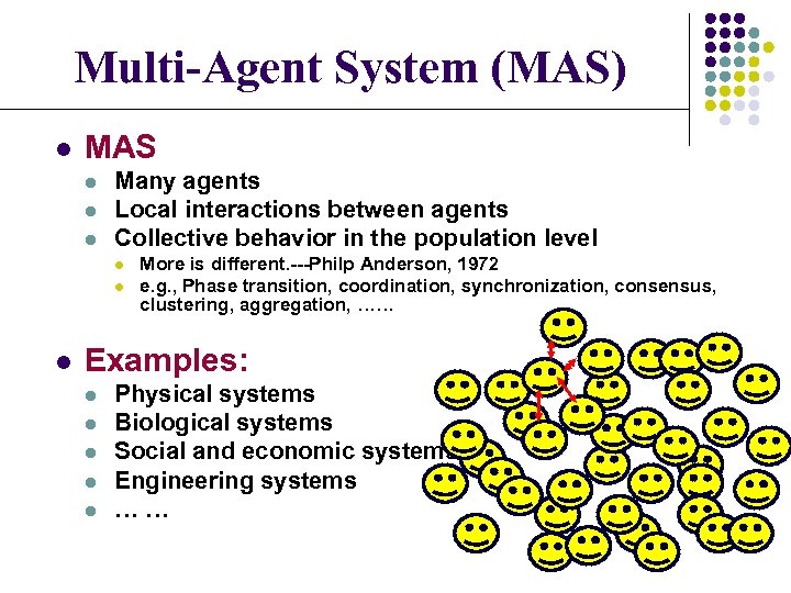Multi-Agent System (MAS) l MAS l l l Many agents Local interactions between agents Collective behavior in the population level l More is different. ---Philp Anderson, 1972 e. g. , Phase transition, coordination, synchronization, consensus, clustering, aggregation, …… Examples: l l l Physical systems Biological systems Social and economic systems Engineering systems ……

Vicsek Model Neighbors: Position: Heading:

Theorem 2 (Jadbabaie et al. , 2003) Joint connectivity of the neighbor graphs on each time interval [th, (t+1)h] with h >0 Synchronization of the linearized Vicsek model Related result: J. N. Tsitsiklis, et al. , IEEE TAC, 1984

Theorem 7 High Density Implies Synchronization For any given system parameters and when the number of agnets n is large, the Vicsek model will synchronize almost surely. This theorem is consistent with the simulation result.

Theorem 8 High density with short distance interaction Let and the velocity satisfy Then for large population, the MAS will synchronize almost surely.

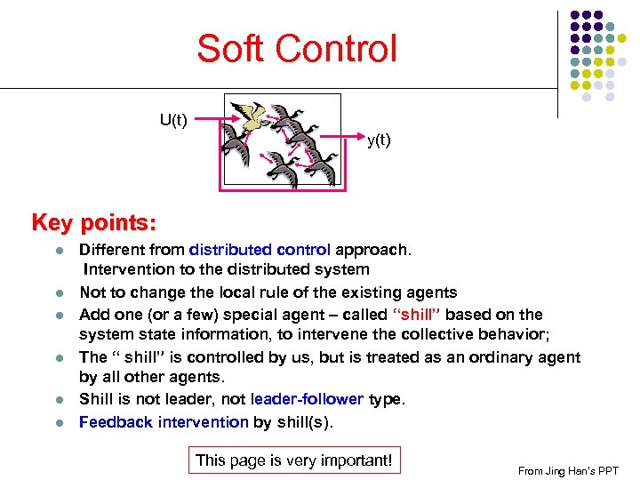Soft Control U(t) y(t) Key points: l l l Different from distributed control approach. Intervention to the distributed system Not to change the local rule of the existing agents Add one (or a few) special agent – called “shill” based on the system state information, to intervene the collective behavior; The “ shill” is controlled by us, but is treated as an ordinary agent by all other agents. Shill is not leader, not leader-follower type. Feedback intervention by shill(s). This page is very important! From Jing Han’s PPT

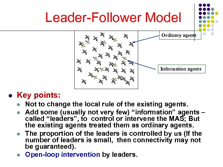Leader-Follower Model Ordinary agents Information agents l Key points: l l Not to change the local rule of the existing agents. Add some (usually not very few) “information” agents – called “leaders”, to control or intervene the MAS; But the existing agents treated them as ordinary agents. The proportion of the leaders is controlled by us (If the number of leaders is small, then connectivity may not be guaranteed). Open-loop intervention by leaders.

Summary In these six lectures, we have talked about: Complex Networks: Topology Collective Behavior of MAS: More is different Game Theory: Interactions Adaptive Systems

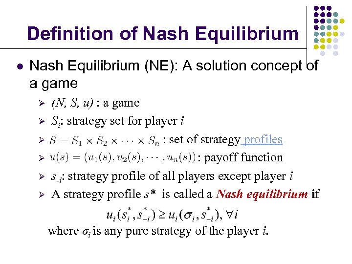Definition of Nash Equilibrium l Nash Equilibrium (NE): A solution concept of a game Ø Ø Ø (N, S, u) : a game Si: strategy set for player i : set of strategy profiles : payoff function s-i: strategy profile of all players except player i A strategy profile s* is called a Nash equilibrium if where σi is any pure strategy of the player i.

Definition of ESS l A strategy x is an ESS if for all y, y x, such that holds for small positiveε.

Summary In these six lectures, we have talked about: Complex Networks: Topology Collective Behavior of MAS: More is different Game Theory: Interactions Adaptive Systems: Adaptation

Other Topics l Self-organizing criticality Earthquakes, fire, sand pile model, Bak-Sneppen model … l Nonlinear dynamics chaos, bifurcation, l Artificial life Tierra model, gene pool, game of life, … l Evolutionary dynamics genetic algorithm, neural network, … l …

Complex systems Ø Ø Not a mature subject No unified framework or universal methods