14f4ad20ab004374b8798f1fb4a03f71.ppt
- Количество слайдов: 34
Lecture Notes: Principles of Probabilities 3/17/2018 BF 330: Risk Management 1
The Principles of Probability. • • • Randomness means that you have no way of knowing which of several possible events will occur in a particular situation at a given time. For example, when we flip a coin, we can't say whether a head or tail will appear. The flipping of the coin is a random experiment. Chance variations means that the event that did occur was not predictable beforehand. That is, when we see that the head is shown after the coin has been flipped, there is no way that such a result could have been predicted in advance. Mathematically speaking, probability is defined as the likelihood of the occurrence of any event in the range of possible chances, or the ratio of the number of favorable chances to the total number of chances, both favorable and unfavorable. 3/17/2018 BF 330: Risk Management 2
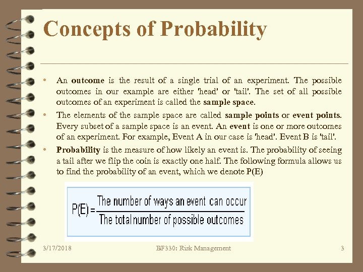
Concepts of Probability • • • An outcome is the result of a single trial of an experiment. The possible outcomes in our example are either 'head' or 'tail'. The set of all possible outcomes of an experiment is called the sample space. The elements of the sample space are called sample points or event points. Every subset of a sample space is an event. An event is one or more outcomes of an experiment. For example, Event A in our case is 'head'. Event B is 'tail'. Probability is the measure of how likely an event is. The probability of seeing a tail after we flip the coin is exactly one half. The following formula allows us to find the probability of an event, which we denote P(E) 3/17/2018 BF 330: Risk Management 3
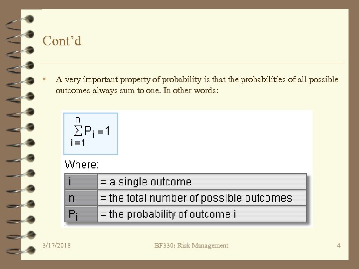
Cont’d • A very important property of probability is that the probabilities of all possible outcomes always sum to one. In other words: 3/17/2018 BF 330: Risk Management 4
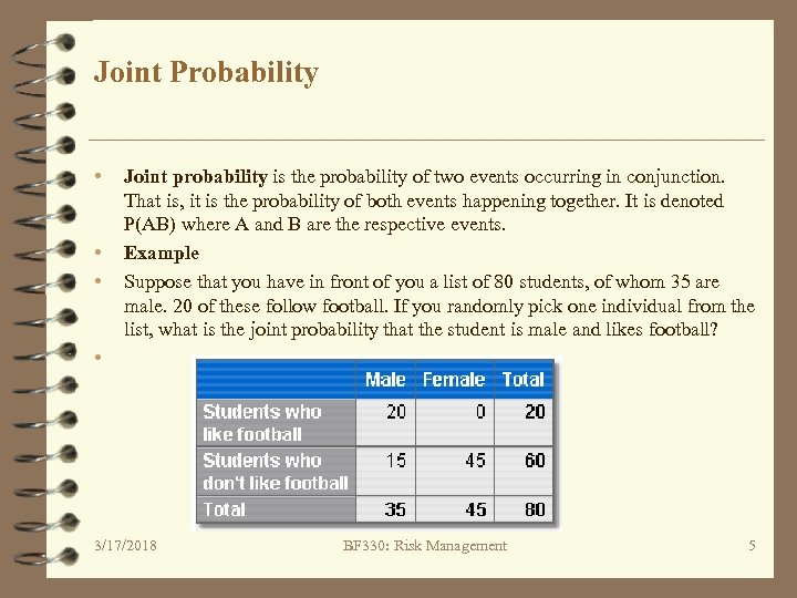
Joint Probability • • Joint probability is the probability of two events occurring in conjunction. That is, it is the probability of both events happening together. It is denoted P(AB) where A and B are the respective events. Example Suppose that you have in front of you a list of 80 students, of whom 35 are male. 20 of these follow football. If you randomly pick one individual from the list, what is the joint probability that the student is male and likes football? 3/17/2018 BF 330: Risk Management 5
Conditional Probability • • • Probabilities can be either conditional or unconditional. So far we have been dealing with unconditional probabilities. In other words, we have answered the question: What is the probability of event P(E)? Here, the probability of the occurrence of event E is unrelated to any other potential outcome. For example, in the example above, we established that the probability of choosing a full-timer from our list of ABC employees was 2/3. This is the unconditional probability, also known as the marginal probability. However, we can also talk about conditional probabilities. Instead of asking the question: What is the probability of event P(E)? , we now ask the question: What is the probability of event E 1 given event E 2? We denote this conditional probability as: P(E 1| E 2). In the example explained earlier, we could have asked: What is the probability of choosing a full-timer given that we have chosen a male employee? 3/17/2018 BF 330: Risk Management 6
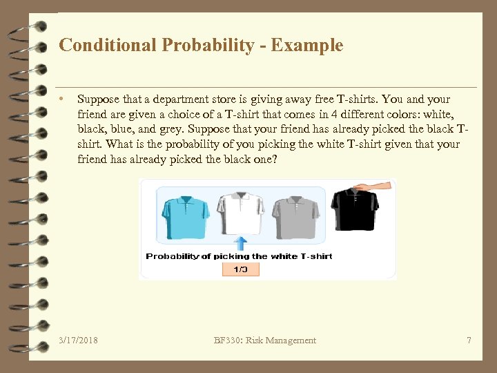
Conditional Probability - Example • Suppose that a department store is giving away free T-shirts. You and your friend are given a choice of a T-shirt that comes in 4 different colors: white, black, blue, and grey. Suppose that your friend has already picked the black Tshirt. What is the probability of you picking the white T-shirt given that your friend has already picked the black one? 3/17/2018 BF 330: Risk Management 7
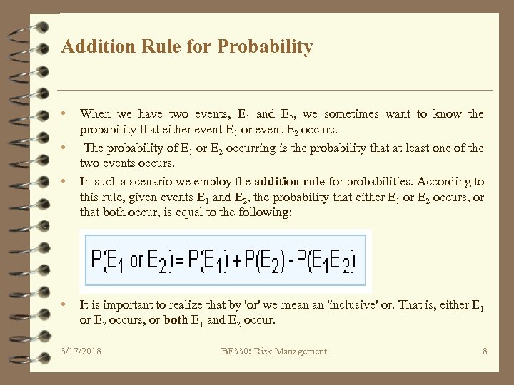
Addition Rule for Probability • • When we have two events, E 1 and E 2, we sometimes want to know the probability that either event E 1 or event E 2 occurs. The probability of E 1 or E 2 occurring is the probability that at least one of the two events occurs. In such a scenario we employ the addition rule for probabilities. According to this rule, given events E 1 and E 2, the probability that either E 1 or E 2 occurs, or that both occur, is equal to the following: It is important to realize that by 'or' we mean an 'inclusive' or. That is, either E 1 or E 2 occurs, or both E 1 and E 2 occur. 3/17/2018 BF 330: Risk Management 8
Example: • Suppose that a few days ago you had an exam in math and another in physics. You do not know yet whether you have passed or failed. You attach a probability of 70% to passing the math exam (event E 1) and a probability of 40% to passing the physics exam (event E 2). The probability that you have passed both exams is 28% (P(E 2) x (P(E 1 E 2)/P(E 2))). What is the probability that you have passed either exam? 3/17/2018 BF 330: Risk Management 9
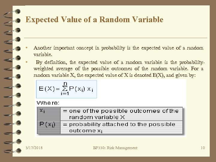
Expected Value of a Random Variable • • Another important concept in probability is the expected value of a random variable. By definition, the expected value of a random variable is the probabilityweighted average of the possible outcomes of the random variable. For a random variable X, the expected value of X is denoted E(X), and given by: 3/17/2018 BF 330: Risk Management 10
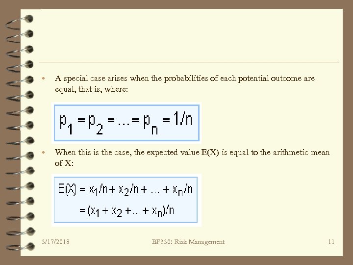
• A special case arises when the probabilities of each potential outcome are equal, that is, where: • When this is the case, the expected value E(X) is equal to the arithmetic mean of X: 3/17/2018 BF 330: Risk Management 11
Example: • • • Suppose that you forecast the GBP/USD exchange rate at the end of next year to be either: 1. 96 with a probability of 65%, or 1. 82 with a probability of 35% What is the expected value of the exchange rate at the end of next year? 3/17/2018 BF 330: Risk Management 12
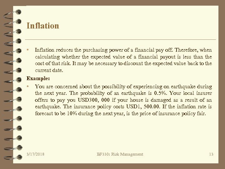
Inflation • Inflation reduces the purchasing power of a financial pay off. Therefore, when calculating whether the expected value of a financial payout is less than the cost of that risk. It may be necessary to discount the expected value back to the current date. Example: • You are concerned about the possibility of experiencing on earthquake during the next year. The probability of an earthquake is 0. 5%. Your local insurer offers to pay you USD 300, 000 if your house is damaged as a result of an earthquake. The insurance policy costs USD 1, 500. If the inflation rate is forecast to be 10% during the next year, is the price of insurance policy fair. 3/17/2018 BF 330: Risk Management 13

3/17/2018 BF 330: Risk Management 14

3/17/2018 BF 330: Risk Management 15

3/17/2018 BF 330: Risk Management 16
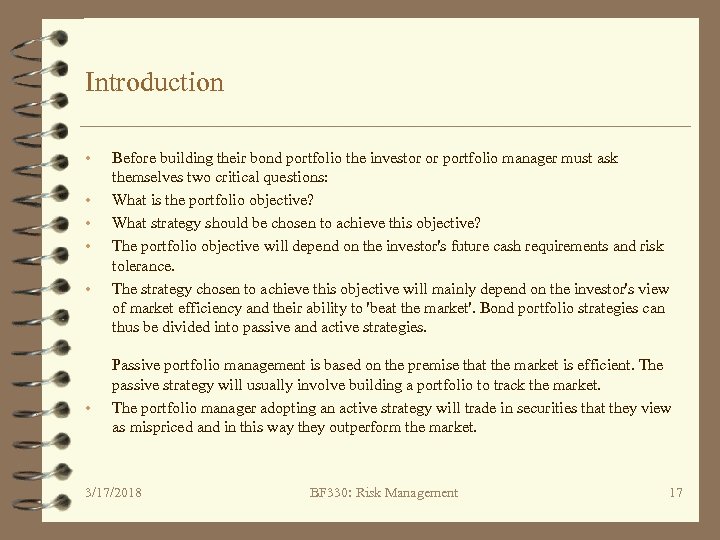
Introduction • • • Before building their bond portfolio the investor or portfolio manager must ask themselves two critical questions: What is the portfolio objective? What strategy should be chosen to achieve this objective? The portfolio objective will depend on the investor's future cash requirements and risk tolerance. The strategy chosen to achieve this objective will mainly depend on the investor's view of market efficiency and their ability to 'beat the market'. Bond portfolio strategies can thus be divided into passive and active strategies. Passive portfolio management is based on the premise that the market is efficient. The passive strategy will usually involve building a portfolio to track the market. The portfolio manager adopting an active strategy will trade in securities that they view as mispriced and in this way they outperform the market. 3/17/2018 BF 330: Risk Management 17
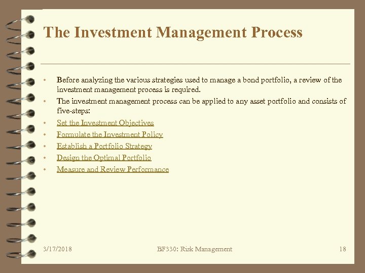
The Investment Management Process • • Before analyzing the various strategies used to manage a bond portfolio, a review of the investment management process is required. The investment management process can be applied to any asset portfolio and consists of five-steps: Set the Investment Objectives Formulate the Investment Policy Establish a Portfolio Strategy Design the Optimal Portfolio Measure and Review Performance 3/17/2018 BF 330: Risk Management 18
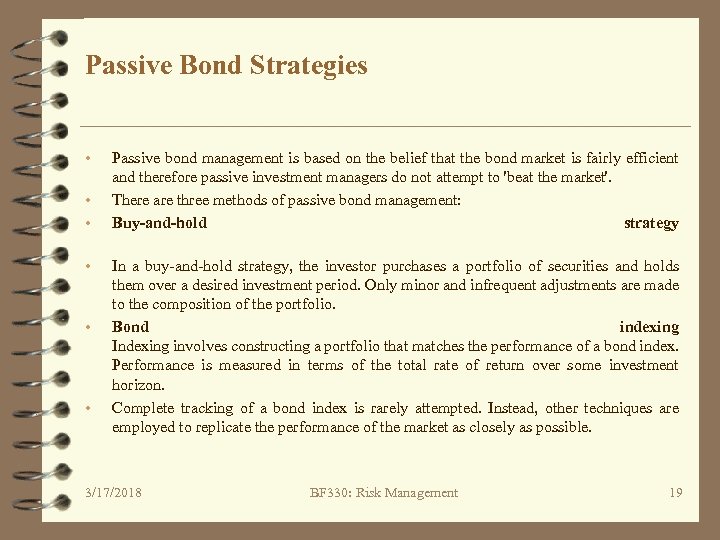
Passive Bond Strategies • • • Passive bond management is based on the belief that the bond market is fairly efficient and therefore passive investment managers do not attempt to 'beat the market'. There are three methods of passive bond management: Buy-and-hold strategy In a buy-and-hold strategy, the investor purchases a portfolio of securities and holds them over a desired investment period. Only minor and infrequent adjustments are made to the composition of the portfolio. Bond indexing Indexing involves constructing a portfolio that matches the performance of a bond index. Performance is measured in terms of the total rate of return over some investment horizon. Complete tracking of a bond index is rarely attempted. Instead, other techniques are employed to replicate the performance of the market as closely as possible. 3/17/2018 BF 330: Risk Management 19
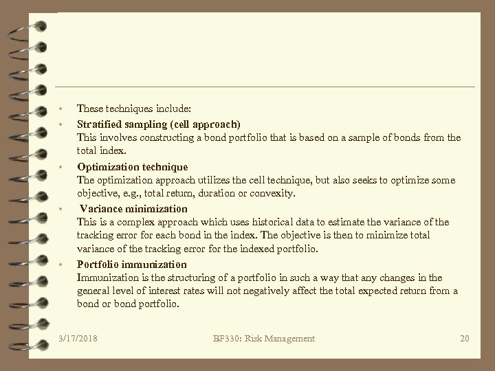
• • • These techniques include: Stratified sampling (cell approach) This involves constructing a bond portfolio that is based on a sample of bonds from the total index. Optimization technique The optimization approach utilizes the cell technique, but also seeks to optimize some objective, e. g. , total return, duration or convexity. Variance minimization This is a complex approach which uses historical data to estimate the variance of the tracking error for each bond in the index. The objective is then to minimize total variance of the tracking error for the indexed portfolio. Portfolio immunization Immunization is the structuring of a portfolio in such a way that any changes in the general level of interest rates will not negatively affect the total expected return from a bond or bond portfolio. 3/17/2018 BF 330: Risk Management 20

Active bond Portfolio Strategies • • • Active bond portfolio strategies are based on the premise that the portfolio manager has superior skill and knowledge relative to other market participants and that the bond market is inefficient. There are four main active bond portfolio strategies: Forecasting interest rates Portfolio managers may position their bond portfolio to reflect their outlook on the future level of interest rates. Identifying mispriced bonds This strategy involves identifying individual bonds that are thought to be under- or overvalued by the market. Yield spread strategies This is a very common strategy which involves positioning the bond portfolio to profit from changes in yield spreads between individual bonds and bond sectors. Yield curve strategies involve positioning a portfolio so as to profit from changes in the shape of the Treasury yield curve. There are three main yield curve strategies a portfolio manager can use to achieve this: 3/17/2018 BF 330: Risk Management 21
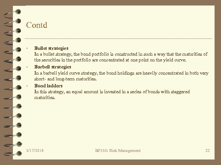
Contd • • • Bullet strategies In a bullet strategy, the bond portfolio is constructed in such a way that the maturities of the securities in the portfolio are concentrated at one point on the yield curve. Barbell strategies In a barbell yield curve strategy, the bond holdings are heavily concentrated in both very short- and long-term maturities. Bond ladders In this strategy, an equal amount is invested in a series of bonds with staggered maturities. 3/17/2018 BF 330: Risk Management 22
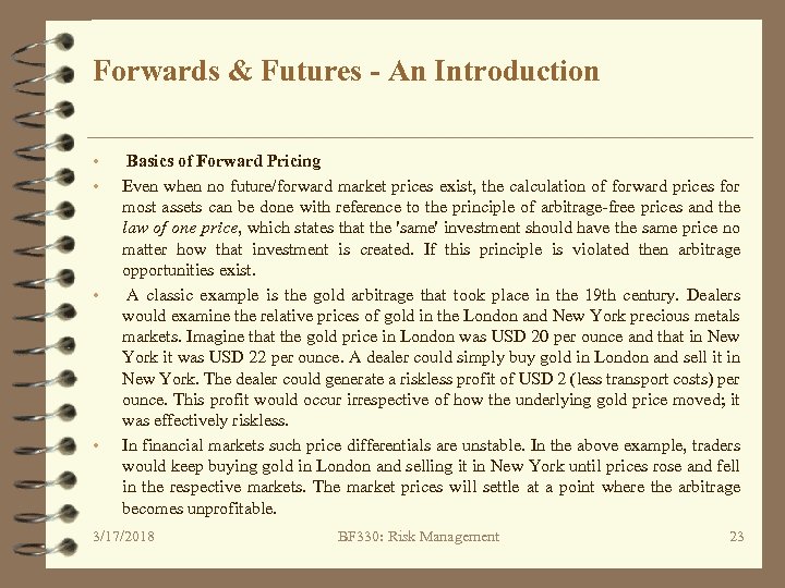
Forwards & Futures - An Introduction • • Basics of Forward Pricing Even when no future/forward market prices exist, the calculation of forward prices for most assets can be done with reference to the principle of arbitrage-free prices and the law of one price, which states that the 'same' investment should have the same price no matter how that investment is created. If this principle is violated then arbitrage opportunities exist. A classic example is the gold arbitrage that took place in the 19 th century. Dealers would examine the relative prices of gold in the London and New York precious metals markets. Imagine that the gold price in London was USD 20 per ounce and that in New York it was USD 22 per ounce. A dealer could simply buy gold in London and sell it in New York. The dealer could generate a riskless profit of USD 2 (less transport costs) per ounce. This profit would occur irrespective of how the underlying gold price moved; it was effectively riskless. In financial markets such price differentials are unstable. In the above example, traders would keep buying gold in London and selling it in New York until prices rose and fell in the respective markets. The market prices will settle at a point where the arbitrage becomes unprofitable. 3/17/2018 BF 330: Risk Management 23
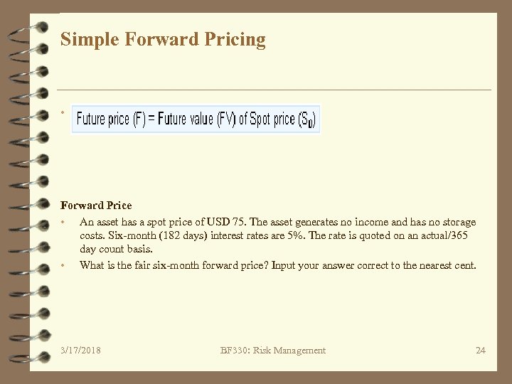
Simple Forward Pricing • Forward Price • An asset has a spot price of USD 75. The asset generates no income and has no storage costs. Six-month (182 days) interest rates are 5%. The rate is quoted on an actual/365 day count basis. • What is the fair six-month forward price? Input your answer correct to the nearest cent. 3/17/2018 BF 330: Risk Management 24
Risk-Free Rate of Interest • • The forward pricing examples mentioned earlier assume that the money can be borrowed or invested at a single rate, at any chosen date. They also implicitly assume that the borrowing/lending is riskless – there is no accounting for counterparty risk. In reality these conditions cannot be satisfied together, although some government securities can be considered riskless. Opportunities do not generally exist for economic agents to both borrow and lend at a single rate in any amount and to any date they choose. However, this ability does effectively exist for major institutions that borrow or lend freely through the interbank deposit market. The risk of default is generally extremely low. Consequently deposit rates, easily observable in the markets, are used as a proxy for risk-free rates 3/17/2018 BF 330: Risk Management 25
Periodic & Continuous Rates • • Another minor complication worth examining at this point is the distinction between interest rates that are quoted using some form of periodic compounding, and continuously-compounded rates. Investments in the market may pay interest on one single date, or else periodically. However, such rates cannot easily be compared. For instance, a 4% rate for a threemonth investment is not the same as a 4% rate for a six-month investment. Furthermore, different market conventions generate different amounts of interest. A 4% three-month deposit rate in the US dollar market is not the same as a 4% three-month deposit in the UK sterling market. This is because USD year fractions are calculated on an actual number of days/360 basis, while GBP rates are calculated on an actual number of days/365 basis. 3/17/2018 BF 330: Risk Management 26
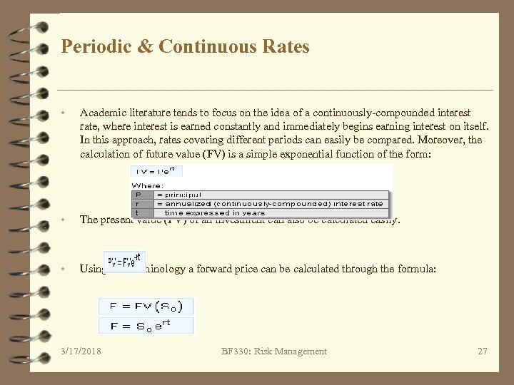
Periodic & Continuous Rates • Academic literature tends to focus on the idea of a continuously-compounded interest rate, where interest is earned constantly and immediately begins earning interest on itself. In this approach, rates covering different periods can easily be compared. Moreover, the calculation of future value (FV) is a simple exponential function of the form: • The present value (PV) of an investment can also be calculated easily. • Using this terminology a forward price can be calculated through the formula: 3/17/2018 BF 330: Risk Management 27
Forward Prices & Forecast Prices • • • The forward price is the price that results from a strategy that can be put in place today. It should not be regarded as an expectation or forecast of where an asset price will actually be at some forward time. Other variables, such as forecasts of supply and demand for a product, or expectations of the future growth of an economy, will be reflected in the spot price of the asset. If the spot price moves then the forward price will move with it. If an agent believes that the future price of an asset will be greater or smaller than the tradable forward price, then a trading opportunity exists, but the potential future price must be compared with the forward, not the spot price. A non income-bearing asset has a spot price of USD 50. 18 -month (exactly 1. 5 year) interest rates are 2% on a continuously-compounded basis. What is the fair 18 -month forward price? Input your answer correct to two decimal places. 3/17/2018 BF 330: Risk Management 28
Exponential function • In mathematics, the exponential function is the function ex, where e is the number (approximately 2. 71828) such that the function ex is its own derivative. The exponential function is used to model phenomena when a constant change in the independent variable gives the same proportional change (i. e. , percent increase or decrease) in the dependent variable. • The natural logarithm is the logarithm to the base e, where e is an irrational constant approximately equal to 2. 71828. The natural logarithm is generally written as ln(x), loge(x) or sometimes, if the base of e is implicit, as simply log(x). • The natural logarithm of a number x (written as ln(x)) is the power to which e would have to be raised to equal x. For example, ln(7. 389. . . ) is 2, because e 2=7. 389. . The natural log of e itself (ln(e)) is 1 because e 1 = e, while the natural logarithm of 1 (ln(1)) is 0, since e 0 = 1. • The natural logarithm can be defined for all positive real numbers a as the area under the curve y = 1/x from 1 to a. The simplicity of this definition, which is matched in many other formulas involving the natural logarithm, leads to the term "natural. " The definition can be extended to non-zero complex numbers, as explained below. • The natural logarithm function, if considered as a real-valued function of a real variable, is the inverse function of the exponential function, leading to the identities: 3/17/2018 BF 330: Risk Management 29 • Like all logarithms, the natural logarithm maps multiplication into addition:
Storage Costs • • • The forward prices generated earlier were calculated with reference to the principle of 'cash and carry'. If the market prices were not equal to theoretical prices, then an arbitrageur could take advantage by replicating the economic performance of a forward contract through a spot transaction in the asset plus the borrowing or lending of money as appropriate. If the asset generated income in the interim, then the fair forward price would fall. Similarly, if there are holding costs involved in storing the asset then the fair forward price will rise. Example A non interest-bearing asset has a spot price of USD 100. It costs 1% per annum (on a simple rate basis) to store the asset. Simple interest rates are 5% per annum. What is the fair one-year forward price? The future value of USD 100 is USD 105, but the forward price cannot be equal to this. Imagine an investor borrows money to buy the asset today. The investor would not only need to repay the future value of USD 100, but would also have to pay the storage costs of 1% (USD 1). If the investor bought the asset today and sold it one-year forward at USD 105 there would be a guaranteed loss and such a price would not be stable. 3/17/2018 BF 330: Risk Management 30
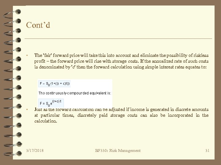
Cont’d • The 'fair' forward price will take this into account and eliminate the possibility of riskless profit – the forward price will rise with storage costs. If the annualized rate of such costs is denominated by 'c' then the forward calculation using simple interest rates equates to: • Just as the forward calculation can be adjusted if income is generated in discrete amounts at particular times, discretely paid storage costs can also be incorporated in the calculation. 3/17/2018 BF 330: Risk Management 31
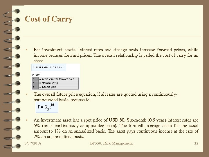
Cost of Carry • For investment assets, interest rates and storage costs increase forward prices, while income reduces forward prices. The overall relationship is called the cost of carry for an asset. • The overall future price equation, if all rates are quoted using a continuouslycompounded basis, reduces to: • An investment asset has a spot price of USD 80. Six-month (0. 5 year) interest rates are 5% (on a continuously-compounded basis). The 6 -month storage costs for the asset amount to 1% on an annualized basis. The asset pays continuous income at the rate of 2% on an annualized basis. 3/17/2018 BF 330: Risk Management 32
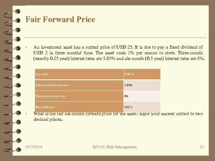
Fair Forward Price • An investment asset has a current price of USD 25. It is due to pay a fixed dividend of USD 2 in three months' time. The asset costs 1% per annum to store. Three-month (exactly 0. 25 year) interest rates are 5. 85% and six-month (0. 5 year) interest rates are 6%. Spot price Three-month interest rate 5. 85% Six-month interest rate 6% Fixed dividend • USD 25 USD 2 What is the fair six-month forward price for the asset? Input your answer correct to two decimal places. 3/17/2018 BF 330: Risk Management 33
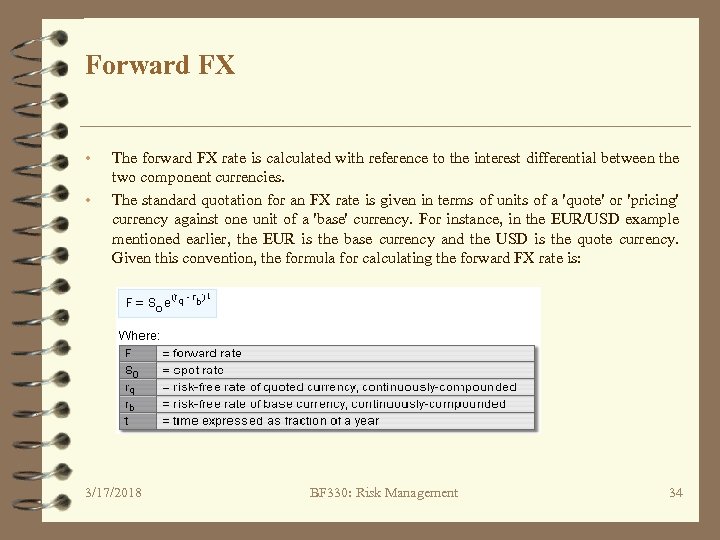
Forward FX • • The forward FX rate is calculated with reference to the interest differential between the two component currencies. The standard quotation for an FX rate is given in terms of units of a 'quote' or 'pricing' currency against one unit of a 'base' currency. For instance, in the EUR/USD example mentioned earlier, the EUR is the base currency and the USD is the quote currency. Given this convention, the formula for calculating the forward FX rate is: 3/17/2018 BF 330: Risk Management 34
14f4ad20ab004374b8798f1fb4a03f71.ppt