Lecture 9 Cost of Capital Mod 7 C

Lecture 9: Cost of Capital Mod 7 C. L. Mattoli 1

Learning outcomes On successful completion of this module you should be able to: n determine a firm’s cost of equity capital n determine a firm’s cost of debt capital n determine a firm’s overall cost of capital n describe some of the problems associated with the firm’s overall cost of capital. n Textbook Chapter 12 2

Intro n n We have spent a lot of time using DFCF evaluation. There are, basically, two variables in that format: forecasted cash flows and a discounting rate. We have also looked into what determines rates of return, in general, like inflation, term, and risk. However, we have not yet given a complete explanation of how discounting rates are determined. 3

Intro n n n In this lecture, we shall discuss the problem of determining required rates of return in the corporate setting. We will find a consistent means of determining discount rates for securities and businesses, and the relationship between the two. This is the cost of capital. Its determination begins in the securities markets. 4

Last Week n n n Last week, we finally examined the risk component of returns, and we found the SML. The SML is a linear relationship between reward, in terms of risk premium over riskless return, and systematic risk, in the form of beta, for securities. That result told us that there has to be only one reward-risk ratio, the reward per unit of risk, i. e. , the slope of the line, in the markets. 5

Last Week n n If that were not true, and a security or portfolio were off the line, then, there would be buying and selling in the marketplace until the assets were moved onto the line. In other words, if an asset had more reward per unit of risk than those on the line, people would buy it. 6

Last Week n n n In buying it, they would bid up the price, which would lower the return until it was finally only as good as the alternatives offered on the line. If it had less reward per unit of risk than those investments on the line, people would sell it, and in selling, the price would go down and the return would increase. We show the situation, graphically, below. 7

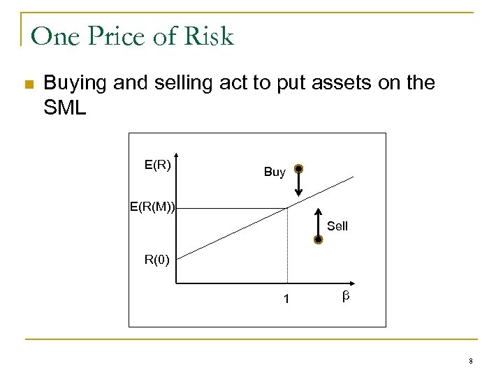One Price of Risk n Buying and selling act to put assets on the SML E(R) Buy E(R(M)) Sell R(0) 1 β 8

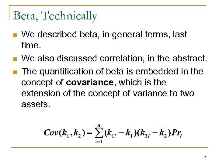Beta, Technically n n n We described beta, in general terms, last time. We also discussed correlation, in the abstract. The quantification of beta is embedded in the concept of covariance, which is the extension of the concept of variance to two assets. 9

Beta, Technically n n n Where the k’s are returns for two assets, in a number of different scenarios. The covariance of returns is a measure of the degree of linear relationship between the two returns, i. e. how they co-vary linearly. However the covariance measure is depends on the unit of measure: dividing it by the product of the two standard deviations removes this dependence and results in a measure (the correlation coefficient) that can only take values between -1 and +1. 10

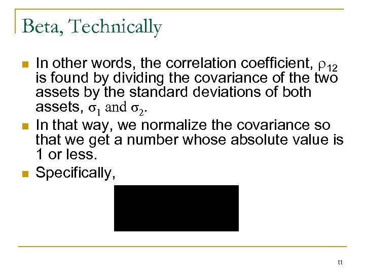Beta, Technically n n n In other words, the correlation coefficient, 12 is found by dividing the covariance of the two assets by the standard deviations of both assets, σ1 and σ2. In that way, we normalize the covariance so that we get a number whose absolute value is 1 or less. Specifically, 11

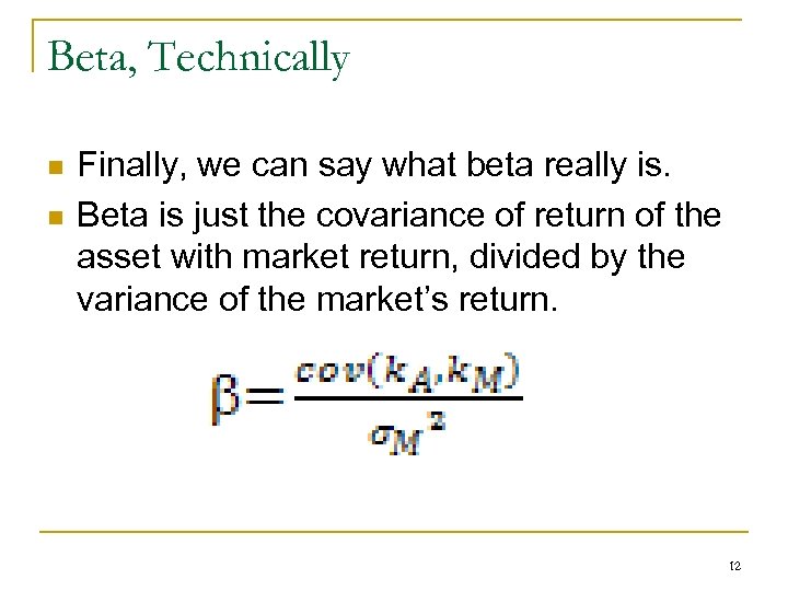Beta, Technically n n Finally, we can say what beta really is. Beta is just the covariance of return of the asset with market return, divided by the variance of the market’s return. 12

From Market to Business n n n According to our CAPM theory, the markets will determine a relationship between return and risk for securities. That result gives the SML with slope the reward per unit risk. If we next consider more general investments, like business projects, the SML offers a benchmark against which to rate reward-risk relationships. 13

From Market to Business n n n In that regard, any investment that a company takes on must offer an expected return that is at least as good as that offered, in the markets, for a particular level of (systematic) risk. If it did not, the firm’s shareholders would be better off, investing on their own, in the markets. Thus, our mandate, as corporate officers, is to try to find investments that offer superior returns to those offered in the markets. 14

From Market to Business n n Such superior investments will have NPV > 0 because they are worth more, based on DFCF, using the return in the market for that level of risk, than we have to pay for them. Looking at it another way, we compare the expected return on the investment (IRR) to the return offered in the market for the same beta. 15

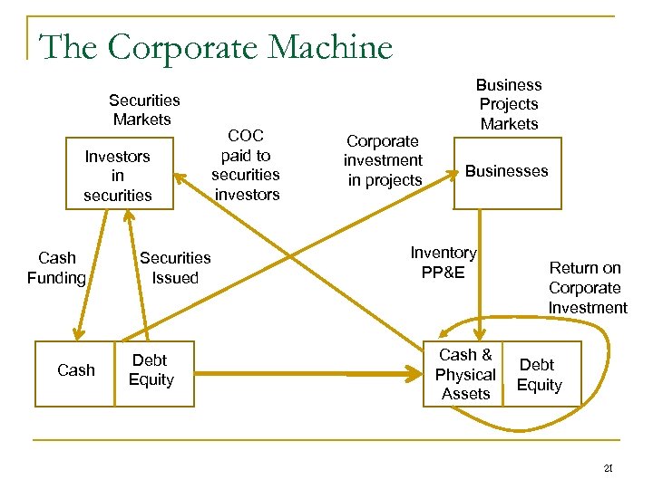
The Corporate Machine n n n We can think of a corporation as a simple machine. When the corporation starts, it is just an empty shell, described on paper, the corporate charter & by-laws. Then, the corporation takes in $$dollars$$, investments from by creditors (debt, BAB’s, bonds, debentures, notes) and owners (common/ordinary and preferred shares of equity capital stock) in corporate securities. 16

The Corporate Machine n n n In return, for the money from these investors in the various securities of the company, the corporation must pay them a return on their investment. It is convenient, as usual, to think of those costs of capital of the corporation for its capital funding in percentage terms. We call each of those percentages that investors require as their returns on the securities, in the market, the cost of capital of each component of capital. 17

The Corporate Machine n n n We also form a weighted average of the components, weighted according to the percentage that each component represents, the weighted average cost of capital (WACC). Now, the corporate shell is filled with money. The next step in the corporate machine is to take that financial capital and invest it in business projects. 18

The Corporate Machine n n Thus, the cash on the left hand side of the balance sheet buys investments in equipment, inventory, and other physical, as opposed to financial, assets to earn a return for the company. Those returns to the company for its physical investments must be sufficient to pay the expected return of the security holders, the cost of capital to the corporation. 19

The Corporate Machine n n n In that regard, the corporate cost of capital becomes a benchmark for evaluating corporate investment in business projects. For the corporation COC = RRR. If the corporation earns a return on its investment in projects equal to the COC, it will earn just enough to pay its investors their required rates of return. In other words, the COC is the BE for corporate investments. We illustrate the corporate machine, in the next slide. 20

The Corporate Machine Securities Markets Investors in securities Cash Funding Cash COC paid to securities investors Securities Issued Debt Equity Corporate investment in projects Business Projects Markets Businesses Inventory PP&E Cash & Physical Assets Return on Corporate Investment Debt Equity 21

The Nature of COC n n n When we talk about RRR for an investment in a business project, we mean that the project must earn a return equal to the RRR to have NPV non-negative. In other words, the firm must earn a RRR equal to COC to compensate its investors for the use of their capital in the project. However, consider a potential investment with zero risk. 22

The Nature of COC To get the proper RRR/COC we turn to the capital markets and use the rate for riskless investment to discount CF’s. n If we have another potential investment with a determined risk level, again, that we look at the market’s RRR for level of risk and use that to discount CF’s. n 23

The Nature of COC To do it any other way would be contrary to the spirit of our understanding of risk and its relationship to return. n Properly, then, COC should be a function of the investment, not the investors, i. e. , COC depends on the use, not the source of funds. n 24

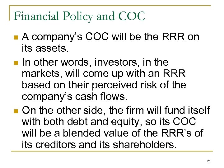Financial Policy and COC A company’s COC will be the RRR on its assets. n In other words, investors, in the markets, will come up with an RRR based on their perceived risk of the company’s cash flows. n On the other side, the firm will fund itself with both debt and equity, so its COC will be a blended value of the RRR’s of its creditors and its shareholders. n 25

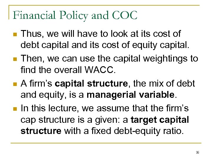Financial Policy and COC n n Thus, we will have to look at its cost of debt capital and its cost of equity capital. Then, we can use the capital weightings to find the overall WACC. A firm’s capital structure, the mix of debt and equity, is a managerial variable. In this lecture, we assume that the firm’s cap structure is a given: a target capital structure with a fixed debt-equity ratio. 26

COC Equity 27

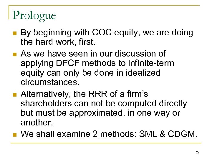Prologue n n By beginning with COC equity, we are doing the hard work, first. As we have seen in our discussion of applying DFCF methods to infinite-term equity can only be done in idealized circumstances. Alternatively, the RRR of a firm’s shareholders can not be computed directly but must be approximated, in one way or another. We shall examine 2 methods: SML & CDGM. 28

COCE: CDGM Approach n n n If we know the market price of equity, there should be an associated RRR. However, to get from P to RRR we need a DFCF equation. The only practical DFCF equation for equity is the CDGM, P 0 = D 0(1+g)/(RE – g). Inverting substituting for D 0, we have RE = D 1/P 0 + g. Since this is the apparent RRR of the firm’s equity investors, it, effectively, becomes the firm’s COC, equity. 29

COCE: CDGM Approach n n n We say effectively, because, properly it is the COC of current shareholders, determined from the secondary markets. If, on the other hand, the firm issued new equity, there would be costs of issuance to pay brokers, investment bankers, lawyers, etc. Those costs would come out of the price investors pay for shares, and would lower the net proceeds received by the firm, raising the actual effective COC return that the firm must cover. 30

CDGM COCE Example n n Assume the market price of XYZ’s shares is $50/share. Assume the firm paid a dividend of $2/share, yesterday, and we expect dividends to grow by 3%/year, forever. Then, D 1 = D 0(1+g) = $2(1. 03) = $2. 06. And RE = COCE = D 1/P 0 + g = $2. 06/$50 + 3% = 7. 12% 31

Estimating G in the CDGM n n n We know price. We want RRR, and the only thing that we need to estimate is g, in the CDGM. The simple ways to do that are to either come up with your own estimate for growth or to use security analysts’ numbers. For example, we can look at past dividends over the past 6 years and find the average growth rate over the period, as we have done in the next slide. 32

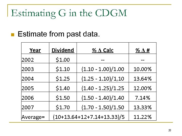Estimating G in the CDGM n Estimate from past data. Year Dividend % Δ Calc %Δ# 2002 $1. 00 -- -- 2003 $1. 10 (1. 10 - 1. 00)/1. 00 10. 00% 2004 $1. 25 (1. 25 - 1. 10)/1, 10 13. 64% 2005 $1. 40 (1. 40 - 1. 25)/1. 25 12. 00% 2006 $1. 50 (1. 50 - 1. 40)/1. 40 7. 14% 2007 $1. 70 (1. 70 - 1. 50)/1. 50 13. 33% (10+13. 64+12+7. 14+13. 33)/5 11. 22% Average= 33

Estimating G in the CDGM n n n Thus, our estimate from these few past years is 11. 22%. Using a longer past will actually be less valuable than a short past since the company might have had a different growth rate in the distant past, and the near past gives a more appropriate estimate. On the other hand, the past is seldom a true precursor of the future. 34

Estimating G in the CDGM n n Securities analysts also might project future dividends or dividend growth rates. You can find those estimates from, e. g. , Zack’s or other services, some for pay, some are free. Again, even those estimates may vary between analysts, so we might take some kind of average of their results. In addition, there are more sophisticated methods of estimating dividend growth, but, in the end, they all root the future in the past. 35

CDGM Pros and Cons n n Although a simple equation, like the CDGM, might not give realistic answers, it is simple, and it is easy to understand. Problems, as you might expect, are numerous. First, if the company pays no dividend, none of our dividend models can be used. Even companies that do pay dividends seldom increase their dividends at some constant annual rate. 36

CDGM Pros and Cons n n Moreover, since the equation is linear in g [i. e. , RE = D 1/P 0 + g], the COCE will increase or decrease by the amount that estimated growth rate is increased or decreased. Finally, the approach explicitly neglects risk, in that there is, e. g. , no adjustment for uncertainty of the growth rate. 37

CDGM Pros and Cons n n In fact, though, since we are using a market price, and we assume that investors in markets adjust prices for risk ) the higher the risk, the lower the price), there is some implicit inclusion of a risk factor in this approach. The next method that we shall look at, the SML approach, which explicitly accounts for risk. 38

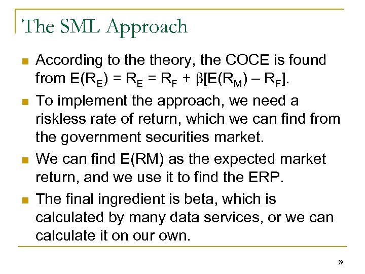The SML Approach n n According to theory, the COCE is found from E(RE) = RE = RF + [E(RM) – RF]. To implement the approach, we need a riskless rate of return, which we can find from the government securities market. We can find E(RM) as the expected market return, and we use it to find the ERP. The final ingredient is beta, which is calculated by many data services, or we can calculate it on our own. 39

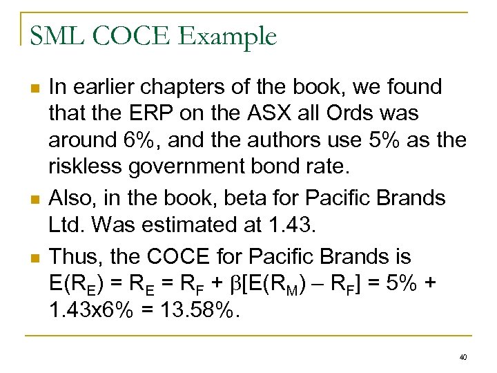SML COCE Example n n n In earlier chapters of the book, we found that the ERP on the ASX all Ords was around 6%, and the authors use 5% as the riskless government bond rate. Also, in the book, beta for Pacific Brands Ltd. Was estimated at 1. 43. Thus, the COCE for Pacific Brands is E(RE) = RE = RF + [E(RM) – RF] = 5% + 1. 43 x 6% = 13. 58%. 40

SLM Pros & Cons n n n The advantage over the CGDM approach is that risk is explicitly included in the computation. Certainly, in the actual markets, investors will adjust their required returns for risk. Then, as long as we can compute a beta for the company and an ERP for the market, we can find an value for COCE. 41

SLM Pros & Cons n n n Another advantage is that the approach does not explicitly need dividends for its calculation, so it will also be applicable to companies that do not pay dividends or even consistent dividends. Of course, all of the variables, beta, ERP, and RF, can change over time. The other problem is that beta calculations can also change over time, and usually several years of data are used to compute them. 42

In the End n n n We can, of course, compare the results for COCE found by both approaches (and any others) to see how well the two agree. As an additional check, we check companies in the same industry to see if we get similar results for either or both methods. Also, just to make sure you are in the right neighborhood, you should check to make sure that the COCE is higher than COC debt and preferred stock, which are less risky securities of the company. 43

COC Debt & Pfd 44

COC Pfd n n n Even though a preferred stock might have an infinite potential life (if it is redeemable, it will have a specific finite life), the dividend is a fixed, non-changing dollar amount. In that regard, it is similar to the situation that we have for debt: there are specific known payments at know future dates. In a preceding section, we valued pfd’s as perpetual annuities. 45

COC Pfd n n n Thus, reversing the process and solving for RRR = COC, given a price, we have COCPfd = RP = D/P 0. That equation is just the current dividend yield on the pfd. In fact, since preferred’s have the same kind of definite payment pattern that is characteristic of debt, we can also get a sense of COC pfd for one preferred stock by comparing to yields of other similar pfd’s in the markets. 46

COC Pfd Example n n n Assume that a preferred stock pays an annual dividend of $10, and it is currently selling in the market for $98. Then, the COCPfd = RP = D/P 0 = $10/$98 = 10. 2%. That should be compared to the COCE and COCD: the value should lie somewhere in between those values because of the relative risks of debt an equity. 47

COC Debt n n Like preferred shares, debt has definite payments at specific times. Unlike perpetual preferred, debt normally has a finite life. The COC debt is just the RRR of creditors of the firm. We might look at the firm’s marginal, i. e. , new, borrowing costs, in the markets for debt. 48

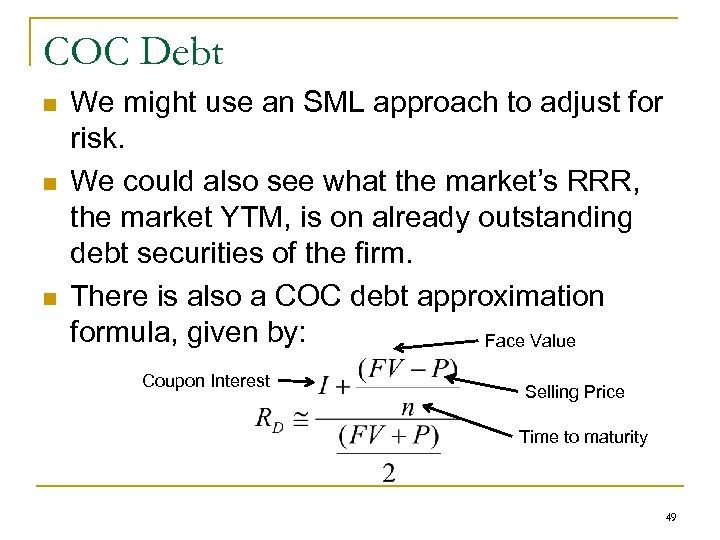COC Debt n n n We might use an SML approach to adjust for risk. We could also see what the market’s RRR, the market YTM, is on already outstanding debt securities of the firm. There is also a COC debt approximation formula, given by: Face Value Coupon Interest Selling Price Time to maturity 49

WACC 50

Capital Weightings n n n Now that we have computed all of the component costs of various forms of capital, we must put them together to form a composite blended COC value. There a number of ways that we could approach the weighting. For example, a firm with privately-placed equity and debt will have only accounting values for capital and weights. 51

Capital Weightings n n n A market-based approach is to take the price times the number of shares or bonds on issue and together all of the market capitalization values for debt, equity and preferred to get the total market value of the firm’s capital. In equations, Total Market Capitalization of capital = V = PE #shares + PP #pfd shares + PD #bonds = E+P+D. Then, the capital weightings for equity, pfd, and debt, respectively, will be: WE = E/V, WP = P/V, and WD = D/V. 52

Capital Weightings They are simply the percentage that each form of capital represents of the total. n These weights are like portfolio weights and are sometimes called the capital structure weights. n Certainly, market values and weights will be better than accounting values. n 53

Capital Weightings However, others argue that these weights will fluctuate with the markets, and that since firms are often shooting for certain target capital weight that those target weights should be the one to use. n Either way, the next step is to combine these capital weights with the COC’s of the various components. n 54

Taxes & WACC n n n In a classical tax system, investors will be concerned with what they really get: after-tax returns. The COC equations for ordinary and preferred equity (at least the CDGM and the Perpetuity), containing, explicitly, dividends, which come out of after-tax income, give after -tax COC’s. On the other hand, interest on debt is a tax deductible expense, so COC debt, using interest payments, is a pre-tax return. 55

Taxes & WACC n n n To get from pre-tax to after-tax interest expense, we use the tax shield method. After-tax interest payment = pre-tax interest – Tx(pre-tax interest) = Pre-tax interest x (1 – T) where T is the corporate tax rate. For example, if the interest rate on debt is 10% on $1 million of bond issue, then PT interest expense is $100, 000, and AT interest is (1 – T)$100, 000 - $70, 000. Then, the effective pre-tax interest rate is $70, 000/$1, 000 = 7%, which is just 10%x(1 – T). 56

Taxes & WACC n n n Since the general rule for pre/after tax interest rate is as above, we can write after tax COC debt = RD(1 – T). In order to have consistency in our construction of WACC, we need all of the component costs to be expressed on an equal footing: either before-tax or after tax. In the classical type of tax system in which dividends and interest are both taxable income to investors, we use after-tax COC’s of the corporation. 57

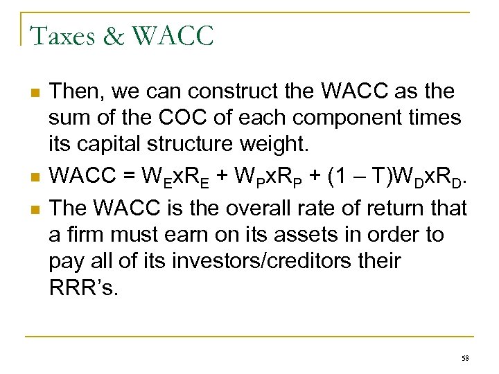Taxes & WACC n n n Then, we can construct the WACC as the sum of the COC of each component times its capital structure weight. WACC = WEx. RE + WPx. RP + (1 – T)WDx. RD. The WACC is the overall rate of return that a firm must earn on its assets in order to pay all of its investors/creditors their RRR’s. 58

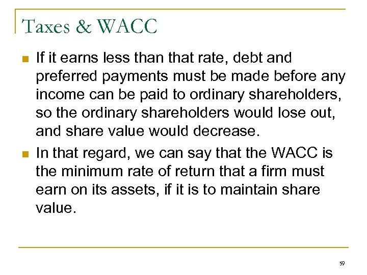Taxes & WACC n n If it earns less than that rate, debt and preferred payments must be made before any income can be paid to ordinary shareholders, so the ordinary shareholders would lose out, and share value would decrease. In that regard, we can say that the WACC is the minimum rate of return that a firm must earn on its assets, if it is to maintain share value. 59

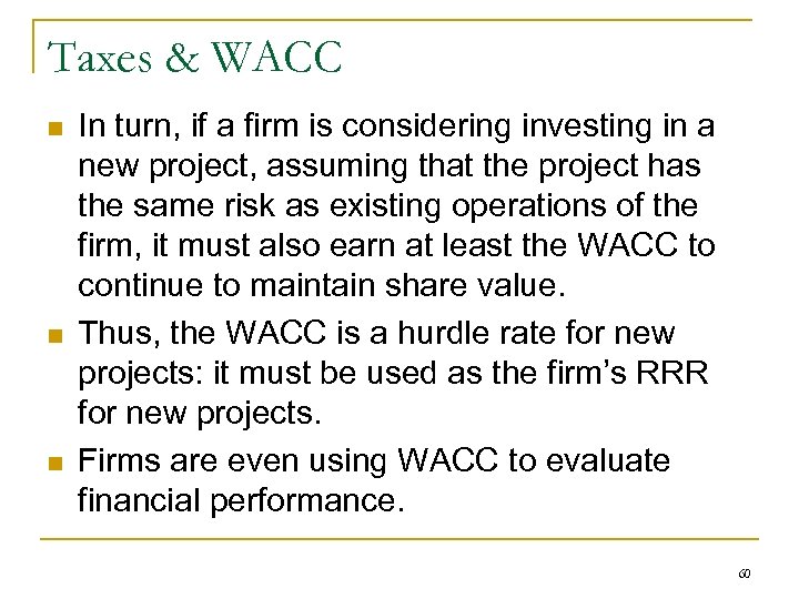Taxes & WACC n n n In turn, if a firm is considering investing in a new project, assuming that the project has the same risk as existing operations of the firm, it must also earn at least the WACC to continue to maintain share value. Thus, the WACC is a hurdle rate for new projects: it must be used as the firm’s RRR for new projects. Firms are even using WACC to evaluate financial performance. 60

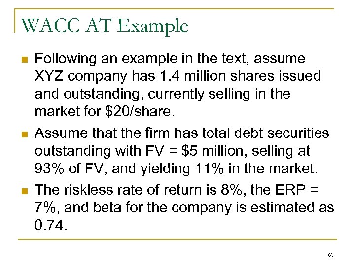WACC AT Example n n n Following an example in the text, assume XYZ company has 1. 4 million shares issued and outstanding, currently selling in the market for $20/share. Assume that the firm has total debt securities outstanding with FV = $5 million, selling at 93% of FV, and yielding 11% in the market. The riskless rate of return is 8%, the ERP = 7%, and beta for the company is estimated as 0. 74. 61

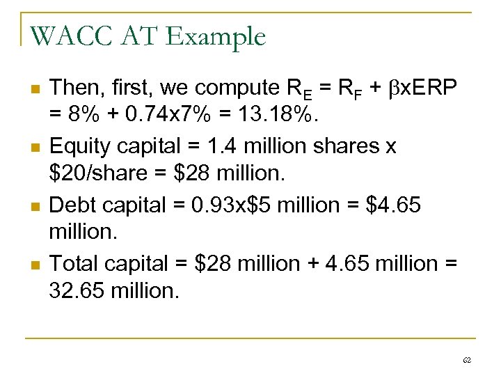WACC AT Example n n Then, first, we compute RE = RF + x. ERP = 8% + 0. 74 x 7% = 13. 18%. Equity capital = 1. 4 million shares x $20/share = $28 million. Debt capital = 0. 93 x$5 million = $4. 65 million. Total capital = $28 million + 4. 65 million = 32. 65 million. 62

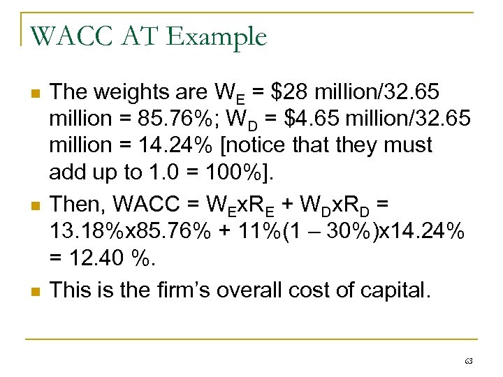WACC AT Example n n n The weights are WE = $28 million/32. 65 million = 85. 76%; WD = $4. 65 million/32. 65 million = 14. 24% [notice that they must add up to 1. 0 = 100%]. Then, WACC = WEx. RE + WDx. RD = 13. 18%x 85. 76% + 11%(1 – 30%)x 14. 24% = 12. 40 %. This is the firm’s overall cost of capital. 63

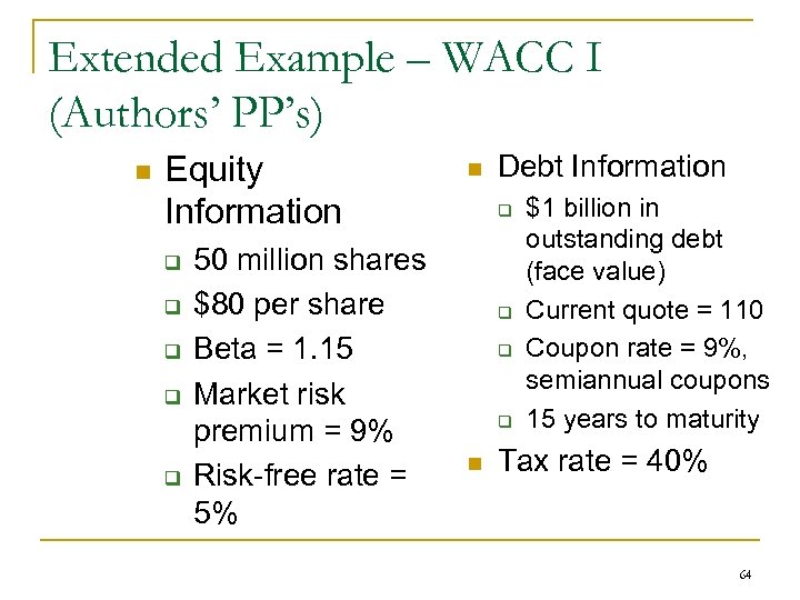Extended Example – WACC I (Authors’ PP’s) n Equity Information q q q 50 million shares $80 per share Beta = 1. 15 Market risk premium = 9% Risk-free rate = 5% n Debt Information q q n $1 billion in outstanding debt (face value) Current quote = 110 Coupon rate = 9%, semiannual coupons 15 years to maturity Tax rate = 40% 64

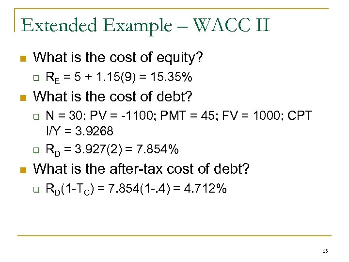Extended Example – WACC II n What is the cost of equity? q n What is the cost of debt? q q n RE = 5 + 1. 15(9) = 15. 35% N = 30; PV = -1100; PMT = 45; FV = 1000; CPT I/Y = 3. 9268 RD = 3. 927(2) = 7. 854% What is the after-tax cost of debt? q RD(1 -TC) = 7. 854(1 -. 4) = 4. 712% 65

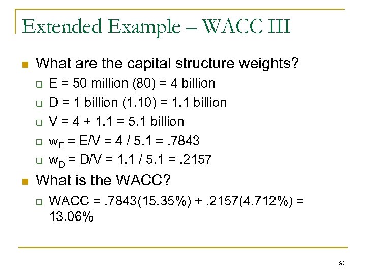Extended Example – WACC III n What are the capital structure weights? q q q n E = 50 million (80) = 4 billion D = 1 billion (1. 10) = 1. 1 billion V = 4 + 1. 1 = 5. 1 billion w. E = E/V = 4 / 5. 1 =. 7843 w. D = D/V = 1. 1 / 5. 1 =. 2157 What is the WACC? q WACC =. 7843(15. 35%) +. 2157(4. 712%) = 13. 06% 66

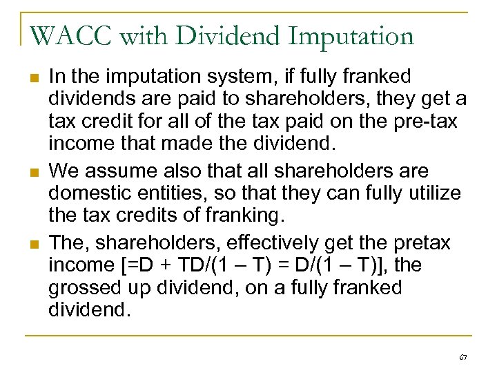WACC with Dividend Imputation n In the imputation system, if fully franked dividends are paid to shareholders, they get a tax credit for all of the tax paid on the pre-tax income that made the dividend. We assume also that all shareholders are domestic entities, so that they can fully utilize the tax credits of franking. The, shareholders, effectively get the pretax income [=D + TD/(1 – T) = D/(1 – T)], the grossed up dividend, on a fully franked dividend. 67

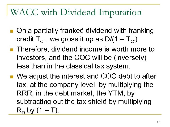WACC with Dividend Imputation n On a partially franked dividend with franking credit TC’ , we gross it up as D/(1 – TC’) Therefore, dividend income is worth more to investors, and the COC will be (inversely) less than in the classical tax system. We adjust the interest and COC debt to after tax, at the company level, by multiplying the RRR, in the debt market, the YTM, by subtracting out the tax shield by multiplying RD by (1 – T). 68

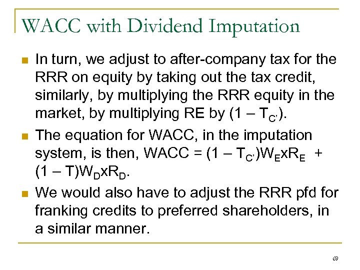WACC with Dividend Imputation n In turn, we adjust to after-company tax for the RRR on equity by taking out the tax credit, similarly, by multiplying the RRR equity in the market, by multiplying RE by (1 – TC’). The equation for WACC, in the imputation system, is then, WACC = (1 – TC’)WEx. RE + (1 – T)WDx. RD. We would also have to adjust the RRR pfd for franking credits to preferred shareholders, in a similar manner. 69

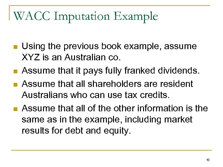WACC Imputation Example n n Using the previous book example, assume XYZ is an Australian co. Assume that it pays fully franked dividends. Assume that all shareholders are resident Australians who can use tax credits. Assume that all of the other information is the same as in the example, including market results for debt and equity. 70

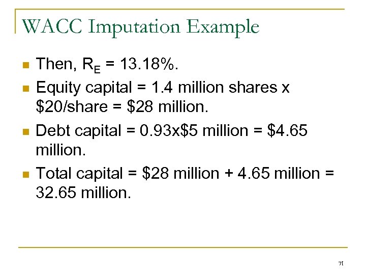WACC Imputation Example n n Then, RE = 13. 18%. Equity capital = 1. 4 million shares x $20/share = $28 million. Debt capital = 0. 93 x$5 million = $4. 65 million. Total capital = $28 million + 4. 65 million = 32. 65 million. 71

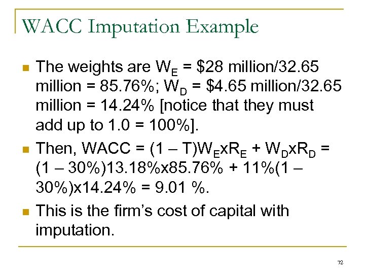WACC Imputation Example n n n The weights are WE = $28 million/32. 65 million = 85. 76%; WD = $4. 65 million/32. 65 million = 14. 24% [notice that they must add up to 1. 0 = 100%]. Then, WACC = (1 – T)WEx. RE + WDx. RD = (1 – 30%)13. 18%x 85. 76% + 11%(1 – 30%)x 14. 24% = 9. 01 %. This is the firm’s cost of capital with imputation. 72

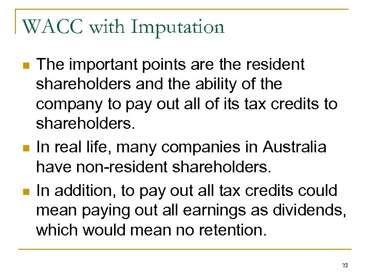WACC with Imputation n The important points are the resident shareholders and the ability of the company to pay out all of its tax credits to shareholders. In real life, many companies in Australia have non-resident shareholders. In addition, to pay out all tax credits could mean paying out all earnings as dividends, which would mean no retention. 73

WACC with Imputation n If the company pays not fully franked dividends, then, we adjust, as in theory part, in a previous slide. Then, We use the franking rate TC’, which can be as small as zero and as large as T = 30%. The focus of the result is that in using WACC for projects, both the project cash flows and the WACC are after-company-tax but before personal investor tax. 74

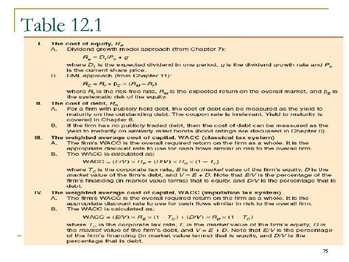Table 12. 1 75

WACC with Dividend Imputation n Note: Peter at USQ has informed me that his lecture and exam will not cover COC with imputation. 76

EVA, SVA & COC n n Another way people are using COC, these days, is to find EVA, economic value added, also called SVA, shareholder value added. It is computed for many companies by Stern Stewart & Co. Find COC, then, multiply by total capital used by the company to get a dollar figure. Then, EVA is that figure minus operating cash flow. 77

WACC Case Studies 78

The warehouse problem n n n Suppose that the company is analyzing a project to renovate its warehouse distribution system at a cost of $50 million. The renovation will result in cost savings of $12 million/year for 6 years. From first principles, we should find a comparable investment in the market, i. e. , similar risk = same risk class. 79

The warehouse problem n n Since the WACC embodies the risk and target cap structure of the firm as a whole, it is appropriate to use it as the discounting rate for projects that replicate the firm’s existing operations, i. e. , are in the same risk class as the firm. Assuming that the warehouse project is an integral operation of the firm, it seems natural to classify it as same risk class as normal operations. 80

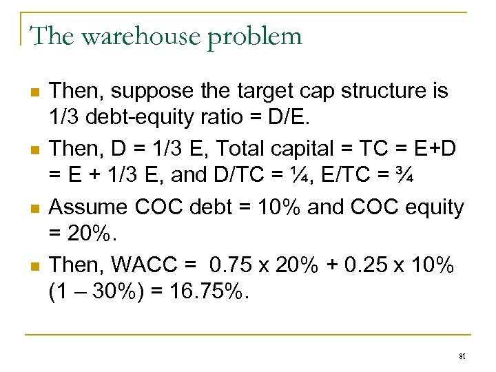The warehouse problem n n Then, suppose the target cap structure is 1/3 debt-equity ratio = D/E. Then, D = 1/3 E, Total capital = TC = E+D = E + 1/3 E, and D/TC = ¼, E/TC = ¾ Assume COC debt = 10% and COC equity = 20%. Then, WACC = 0. 75 x 20% + 0. 25 x 10% (1 – 30%) = 16. 75%. 81

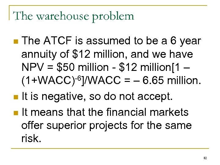The warehouse problem The ATCF is assumed to be a 6 year annuity of $12 million, and we have NPV = $50 million - $12 million[1 – (1+WACC)-6]/WACC = – 6. 65 million. n It is negative, so do not accept. n It means that the financial markets offer superior projects for the same risk. n 82

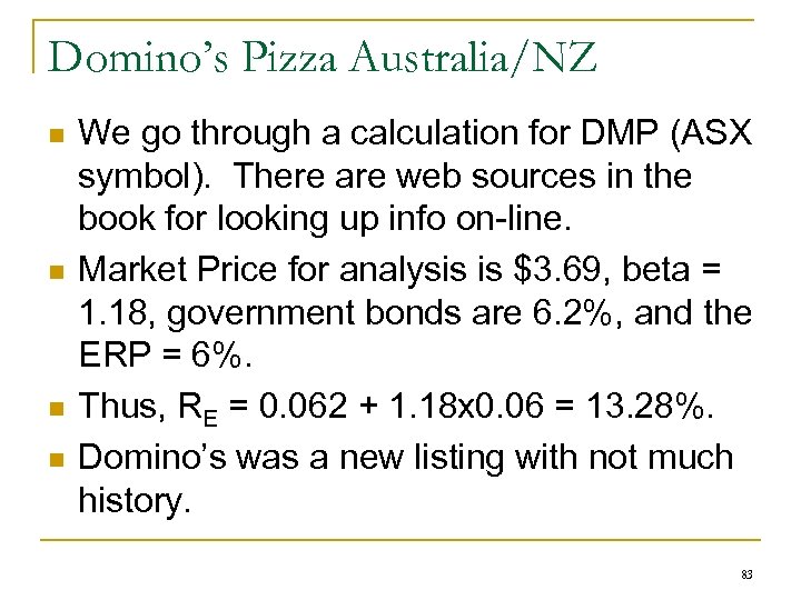Domino’s Pizza Australia/NZ n n We go through a calculation for DMP (ASX symbol). There are web sources in the book for looking up info on-line. Market Price for analysis is $3. 69, beta = 1. 18, government bonds are 6. 2%, and the ERP = 6%. Thus, RE = 0. 062 + 1. 18 x 0. 06 = 13. 28%. Domino’s was a new listing with not much history. 83

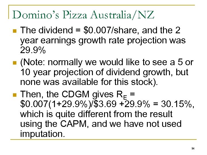Domino’s Pizza Australia/NZ n n n The dividend = $0. 007/share, and the 2 year earnings growth rate projection was 29. 9% (Note: normally we would like to see a 5 or 10 year projection of dividend growth, but none was available for this stock). Then, the CDGM gives RE = $0. 007(1+29. 9%)/$3. 69 +29. 9% = 30. 15%, which is quite different from the result using the CAPM, and we have not used imputation. 84

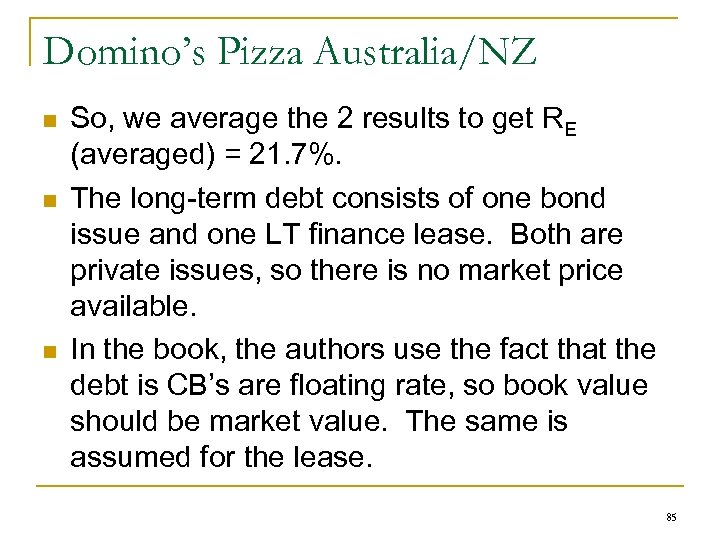Domino’s Pizza Australia/NZ n n n So, we average the 2 results to get RE (averaged) = 21. 7%. The long-term debt consists of one bond issue and one LT finance lease. Both are private issues, so there is no market price available. In the book, the authors use the fact that the debt is CB’s are floating rate, so book value should be market value. The same is assumed for the lease. 85

Domino’s Pizza Australia/NZ n n n We assume that the second table on page 379 is the correct one (there is a conflict between the values of yield for the financing lease), and the weighted average COC debt is 6. 63%. There are $221. 6 million market value of equity, and $14. 495 million in debt; total cap = $236. 1 million. Thus WACC = (221. 6/236. 1)21. 7% + (14. 5/236. 1)6. 63(70%) = 20. 7% 86

Other COC Concepts 87

Divisional & Project COC’s n n n For projects similar to the firm’s existing operations, the WACC is a proper benchmark. However, other projects might require a different discounting rate. If we use WACC to evaluate projects with risks different from the average firm risk, it will lead to improper decisions. 88

Divisional & Project COC’s Note, even a new line of business will be riskier than the firm’s average risk. n From SML theory, we know that NPV > 0 projects lie above the line. n However, using WACC might lead to accepting projects below the line and rejecting projects above the line. n We illustrate this, in the next slide. n 89

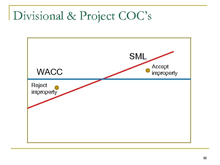Divisional & Project COC’s SML WACC Accept improperly Reject improperly 90

Divisional & Project COC’s n n A company, like a conglomerate, may have divisions with vastly different risks, like military hardware and canned soup. Then, the company might, quite naturally, think of finding appropriate COC’s for each division. Riskier divisions will have a higher COC hurdle and less risky divisions, a lower rate. In sum, the weighted divisional COC must equal the firm’s average perceived risk. 91

Pure Play Approach n n n One way that it might be possible to come up with risk and return for a project or a division is the pure play approach. In this approach, we look to the market for companies that are in the same business or in the same risk class. For example, if our project or division is a cell phone maker, we can look at the market RRR for cell phone makers. 92

Subjective Approach n n n Often companies will take the WACC as an average value for average projects, and will subjectively determine appropriate rate for less and more risky projects. One reason that a company might settle for this method is the cost of trying to figure out perfect rates, inavailability of pure plays to look to, or for simplicity. This will, however, lead to a better system than pure WACC, as illustrated, below. 93

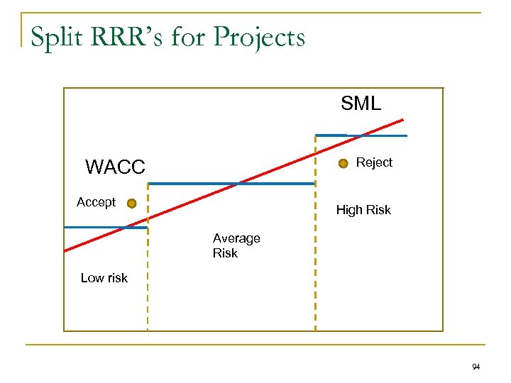Split RRR’s for Projects SML Reject WACC Accept High Risk Average Risk Low risk 94

Learning activity Attempt all of the critical thinking and concepts review questions on pages 385 to 386. n Attempt questions and problems 1, 3, 4, 5, 8, 9, 15, 19 and 30 n 95

END 96