Lecture 9 Chapters 11 12 Repeated Measures t

Lecture 9: Chapters 11 &12 Repeated Measures t - statistic & Estimation

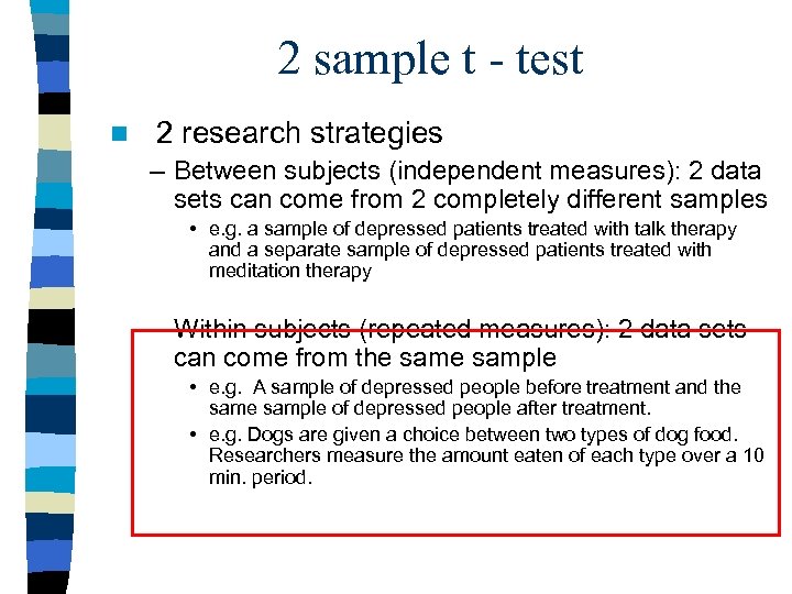2 sample t - test n 2 research strategies – Between subjects (independent measures): 2 data sets can come from 2 completely different samples • e. g. a sample of depressed patients treated with talk therapy and a separate sample of depressed patients treated with meditation therapy – Within subjects (repeated measures): 2 data sets can come from the sample • e. g. A sample of depressed people before treatment and the sample of depressed people after treatment. • e. g. Dogs are given a choice between two types of dog food. Researchers measure the amount eaten of each type over a 10 min. period.

Repeated Measures Stats n Within subjects: a single sample of individuals is measured more than once on the same dependent variable. The same subjects are used in all treatment conditions n Matched sample: 2 separate samples of subjects, but each individual in one sample is matched with a subject in the other sample. – e. g. match subjects across several variables like age, income, education, sex. In this chapter we are going to focus on repeated measures b/c they are more common than matched subjects, but the same statistical techniques apply.

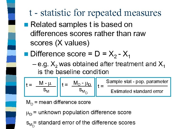t - statistic for repeated measures n Related samples t is based on differences scores rather than raw scores (X values) n Difference score = D = X 2 - X 1 – e. g. X 2 was obtained after treatment and X 1 is the baseline condition M- t= s. M t= MD - D s. MD t= Sample stat - pop. parameter Estimated standard error MD = mean difference score D = unknown population difference score s. M = standard error of the difference scores D

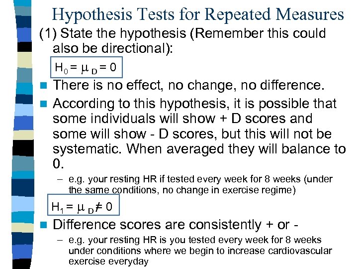Hypothesis Tests for Repeated Measures (1) State the hypothesis (Remember this could also be directional): H 0 = D = 0 n There is no effect, no change, no difference. n According to this hypothesis, it is possible that some individuals will show + D scores and some will show - D scores, but this will not be systematic. When averaged they will balance to 0. – e. g. your resting HR if tested every week for 8 weeks (under the same conditions, no change in exercise regime) H 1 = D = 0 n Difference scores are consistently + or – e. g. your resting HR is you tested every week for 8 weeks under conditions where we begin to increase cardiovascular exercise everyday

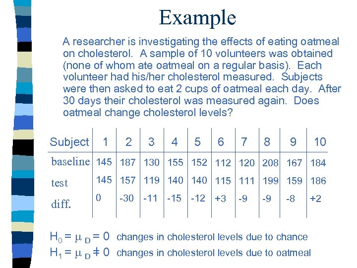Example A researcher is investigating the effects of eating oatmeal on cholesterol. A sample of 10 volunteers was obtained (none of whom ate oatmeal on a regular basis). Each volunteer had his/her cholesterol measured. Subjects were then asked to eat 2 cups of oatmeal each day. After 30 days their cholesterol was measured again. Does oatmeal change cholesterol levels? Subject 1 2 3 4 5 6 7 8 9 10 baseline 145 187 130 155 152 112 120 208 167 184 test diff. 145 157 119 140 115 111 199 159 186 0 -30 -11 -15 -12 +3 -9 -9 -8 +2 H 0 = D = 0 changes in cholesterol levels due to chance H 1 = D = 0 changes in cholesterol levels due to oatmeal

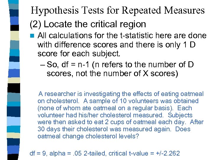Hypothesis Tests for Repeated Measures (2) Locate the critical region n All calculations for the t-statistic here are done with difference scores and there is only 1 D score for each subject. – So, df = n-1 (n refers to the number of D scores, not the number of X scores) A researcher is investigating the effects of eating oatmeal on cholesterol. A sample of 10 volunteers was obtained (none of whom ate oatmeal on a regular basis). Each volunteer had his/her cholesterol measured. Subjects were then asked to eat 2 cups of oatmeal each day. After 30 days their cholesterol was measured again. Does oatmeal change cholesterol levels? df = 9, alpha =. 05 2 -tailed, critical t-value = +/-2. 262

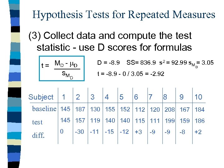Hypothesis Tests for Repeated Measures (3) Collect data and compute the test statistic - use D scores formulas t = MD - D s. M Subject 1 D = -8. 9 SS= 836. 9 s 2 = 92. 99 s. M = 3. 05 D t = -8. 9 - 0 / 3. 05 = -2. 92 D 2 3 4 5 6 7 8 9 10 baseline 145 187 130 155 152 112 120 208 167 184 test diff. 145 157 119 140 115 111 199 159 186 0 -30 -11 -15 -12 +3 -9 -9 -8 +2

Hypothesis Tests for Repeated Measures (4) Make a decision Our t value is -2. 92 and our t-critical value was 2. 262, so we can reject the null hypothesis! Eating oatmeal significantly reduces cholesterol, t(9) = -2. 92, p <. 05

Directional Hypothesis Test for Repeated Measures n What would change in our previous example if we had predicted that oatmeal would lower cholesterol levels? – State hypothesis H 0 = D 0 cholesterol levels are not reduced after eating oatmeal H 1 = D < 0 cholesterol levels are reduced after eating oatmeal – Locate critical region df = n-1 df = 9 Alpha =. 05 1 -tailed Critical value = -1. 833

Measuring Effect Size nd = mean difference / standard deviation d = DM / s From our oatmeal example: DM = -2. 92 s 2 = 92. 99 s = 9. 62 D = 2. 92 / 9. 62 =. 3 Medium effect

Measuring Effect Size n r 2 = t 2 / (t 2 + df) r 2 = -2. 922 / (-2. 922 + 9) r 2 =. 49 or 49 % of the variance Large effect size using this measure

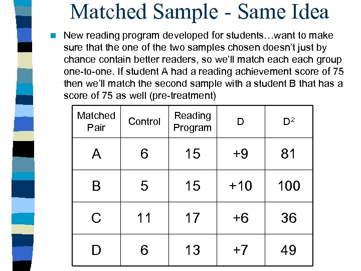Matched Sample - Same Idea n New reading program developed for students…want to make sure that the one of the two samples chosen doesn’t just by chance contain better readers, so we’ll match each group one-to-one. If student A had a reading achievement score of 75 then we’ll match the second sample with a student B that has a score of 75 as well (pre-treatment) Matched Pair Control Reading Program D D 2 A 6 15 +9 81 B 5 15 +10 100 C 11 17 +6 36 D 6 13 +7 49

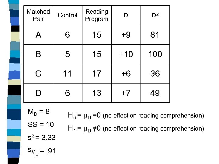Matched Pair Control Reading Program D D 2 A 6 15 +9 81 B 5 15 +10 100 C 11 17 +6 36 D 6 13 +7 49 MD = 8 H 0 = D =0 (no effect on reading comprehension) SS = 10 H 1 = D =0 (no effect on reading comprehension) s 2 = 3. 33 s. M =. 91 D

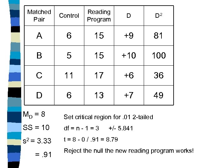Matched Pair Control Reading Program D D 2 A 6 15 +9 81 B 5 15 +10 100 C 11 17 +6 36 D 6 13 +7 49 MD = 8 Set critical region for. 01 2 -tailed SS = 10 df = n - 1 = 3 s 2 = 3. 33 t = 8 - 0 /. 91 = 8. 79 =. 91 +/- 5. 841 Reject the null the new reading program works!

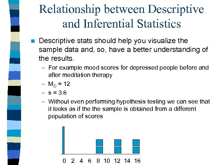Relationship between Descriptive and Inferential Statistics n Descriptive stats should help you visualize the sample data and, so, have a better understanding of the results. – For example mood scores for depressed people before and after meditation therapy – MD = 12 – s = 3. 6 – Without even performing hypothesis testing we can see that it looks as if the sample is obtained from a different population of scores 0 2 4 6 8 10 12 14 16

Advantages to Repeated Measures n Good when only a small N is available – e. g. patient populations, rare species, etc. n Good for questions that are looking for changes across time – Developmental questions – Learning questions n No worry about individual differences – No worries about the difference simply being due to individuals (e. g. in a learning study that one group was just smarter than the other group) – Decreases sample variance (which remember the higher the variance the more difficult it becomes to see a pattern in our data)

Disadvantages n Carryover effects - participant’s response in the second treatment is altered by lingering effects of the first treatment – e. g. administering the second drug too soon after the first n Progressive error - participant’s performance changes consistently over time – e. g. a participant improves over time simply due to practice n Counterbalancing the order treatment can help with these problems – e. g. Subject 1 gets treatment 1 first then treatment 2. Then subject 2 gets treatment 2 first then treatment 1.

Estimation - Another Inferential Statistical Procedure n Hypothesis testing lets us know if a particular sample came from a particular population. It helps us evaluate the effect of the treatment. The treatment either has an effect or it doesn’t. – Eating oatmeal does lower cholesterol n Estimation is the process of using sample data to actually estimate the values for population parameters. – So, it will determine the value of the population mean after treatment. It will estimate how much effect the treatment had. How big or small the effect is.

Estimation n The use of samples to estimate the population is quite common – 42% of the population supports the president – 8% of UA students are members of the Green Party – 34% of Americans are homeowners NOTE: We’ve already done estimation before. We know how to estimate the population variance from the sample variance. Using df.

2 - Types of Estimation We also know how to estimate the SE, so we know what the average distance from our sample mean to our population mean is. So, we can begin to estimate our population mean… n Point estimation - a specific value using 1 number to estimate the population mean. n – If I were to estimate the weight of my dog I’d say 100 lbs. n Interval estimation / Confidence intervals - uses a range of values to estimate the population mean. Interval estimates are usually accompanied by the probability of obtaining that range of values. This probability information is called a level of confidence. – If I were to estimate the weight of my dog I might say between 90 and 110 lbs.

When should we estimate? (1) After a hypothesis test when H 0 is rejected. This is the case where we know there is a treatment effect, but we want to know how much. (Like the oatmeal example. ) (2) When you know there is an effect, but you want to know how much. – For instance, we probably know that tutoring will improve grades. However, tutoring is $25 / hour. We want to know how much our grade will improve to figure out if the cost for us will be justified. (3) We want basic information about a population – For instance, we want to know the average number of times college students eat pizza each week. – We want to know about how many people support the war in Iraq.

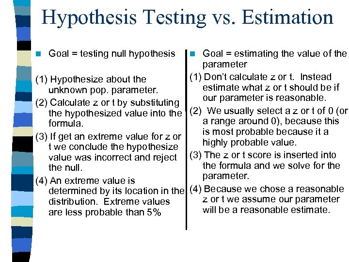Hypothesis Testing vs. Estimation Goal = estimating the value of the parameter (1) Don’t calculate z or t. Instead (1) Hypothesize about the estimate what z or t should be if unknown pop. parameter. our parameter is reasonable. (2) Calculate z or t by substituting the hypothesized value into the (2) We usually select a z or t of 0 (or a range around 0), because this formula. is most probable because it a (3) If get an extreme value for z or highly probable value. t we conclude the hypothesize value was incorrect and reject (3) The z or t score is inserted into the formula and we solve for the null. parameter. (4) An extreme value is determined by its location in the (4) Because we chose a reasonable z or t we assume our parameter distribution. Extreme values will be a reasonable estimate. are less probable than 5% n Goal = testing null hypothesis n

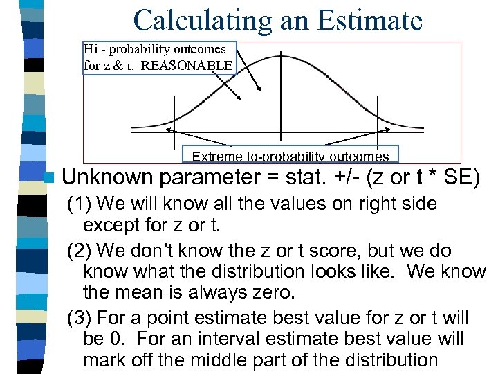Calculating an Estimate Hi - probability outcomes for z & t. REASONABLE n Unknown Extreme lo-probability outcomes parameter = stat. +/- (z or t * SE) (1) We will know all the values on right side except for z or t. (2) We don’t know the z or t score, but we do know what the distribution looks like. We know the mean is always zero. (3) For a point estimate best value for z or t will be 0. For an interval estimate best value will mark off the middle part of the distribution

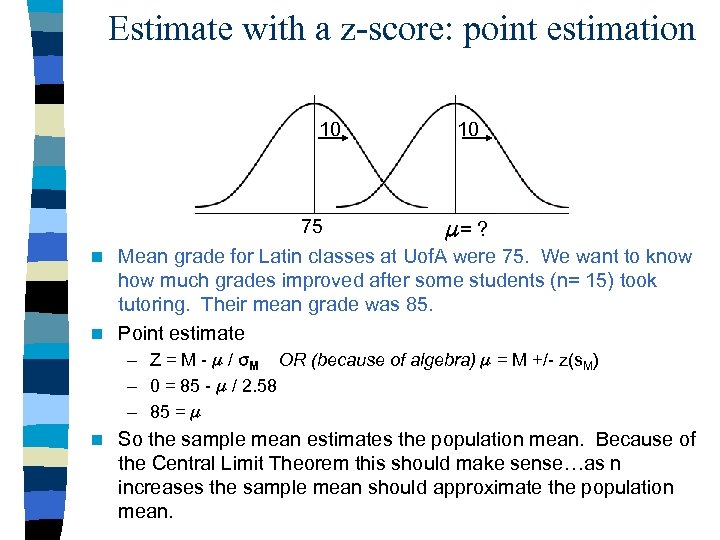Estimate with a z-score: point estimation 10 75 10 = ? Mean grade for Latin classes at Uof. A were 75. We want to know how much grades improved after some students (n= 15) took tutoring. Their mean grade was 85. n Point estimate n – Z = M - / M OR (because of algebra) = M +/- z(s. M) – 0 = 85 - / 2. 58 – 85 = n So the sample mean estimates the population mean. Because of the Central Limit Theorem this should make sense…as n increases the sample mean should approximate the population mean.

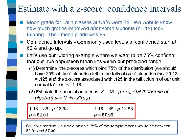Estimate with a z-score: confidence intervals Mean grade for Latin classes at Uof. A were 75. We want to know how much grades improved after some students (n= 15) took tutoring. Their mean grade was 85. n Confidence intervals - Commonly used levels of confidence start at 60% and go up. n Let’s use our tutoring example where we want to be 75% confident that our true population mean lies within our predicted range. n (1) Determine the z-scores which bind 75% of the distribution (we should have 25% of the distribution left in the tails of our distribution (so. 25 / 2 =. 125 and the z-score associated with. 125 in the tail column of our unit normal table is +/- 1. 16 (2) Estimate the population means: Z = M - / M OR (because of algebra) = M +/- z*(s. M) 1. 16 = 85 - / 2. 58 = 82. 01 -1. 16 = 85 - / 2. 58 = 87. 99 So, if we randomly pulled a sample 75% of the sample means would be between 82. 01 and 87. 99

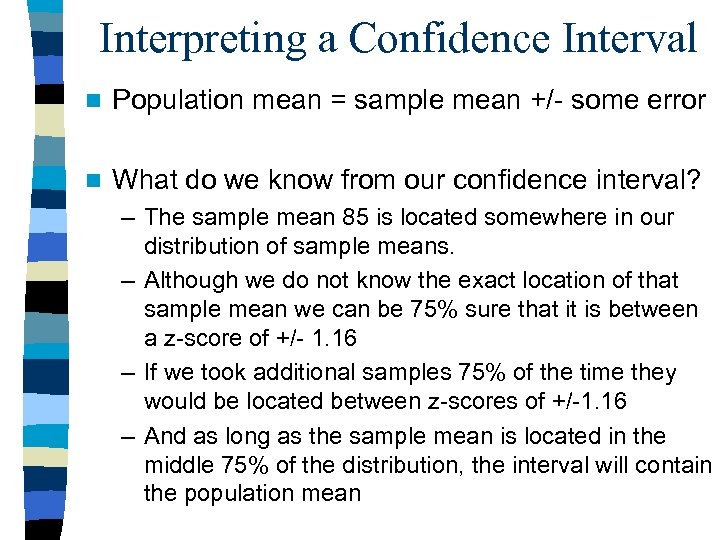Interpreting a Confidence Interval n Population mean = sample mean +/- some error n What do we know from our confidence interval? – The sample mean 85 is located somewhere in our distribution of sample means. – Although we do not know the exact location of that sample mean we can be 75% sure that it is between a z-score of +/- 1. 16 – If we took additional samples 75% of the time they would be located between z-scores of +/-1. 16 – And as long as the sample mean is located in the middle 75% of the distribution, the interval will contain the population mean

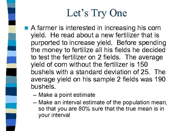Let’s Try One n A farmer is interested in increasing his corn yield. He read about a new fertilizer that is purported to increase yield. Before spending the money to fertilize all his fields he decided to test the fertilizer on 2 fields. The average yield of corn without the fertilizer is 150 bushels with a standard deviation of 25. The average yield on his sample 2 fields was 190 bushels. – Make a point estimate – Make an interval estimate of the population mean, so that you are 80% sure that the true mean is in your interval

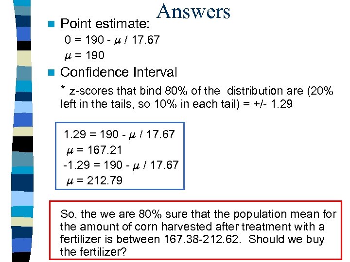Answers n Point estimate: 0 = 190 - / 17. 67 = 190 n Confidence Interval * z-scores that bind 80% of the distribution are (20% left in the tails, so 10% in each tail) = +/- 1. 29 = 190 - / 17. 67 = 167. 21 -1. 29 = 190 - / 17. 67 = 212. 79 So, the we are 80% sure that the population mean for the amount of corn harvested after treatment with a fertilizer is between 167. 38 -212. 62. Should we buy the fertilizer?

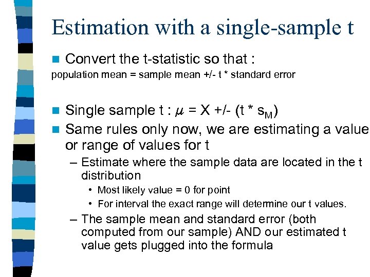Estimation with a single-sample t n Convert the t-statistic so that : population mean = sample mean +/- t * standard error Single sample t : = X +/- (t * s. M) n Same rules only now, we are estimating a value or range of values for t n – Estimate where the sample data are located in the t distribution • Most likely value = 0 for point • For interval the exact range will determine our t values. – The sample mean and standard error (both computed from our sample) AND our estimated t value gets plugged into the formula

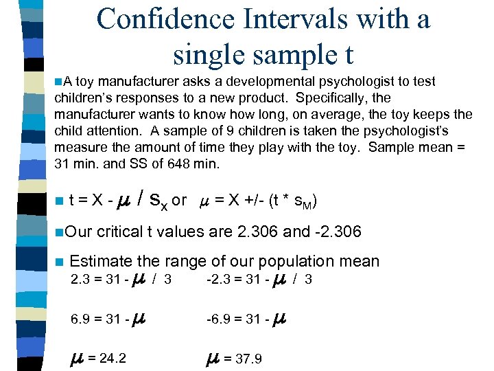
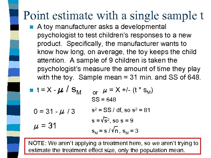Point estimate with a single sample t n n A toy manufacturer asks a developmental psychologist to test children’s responses to a new product. Specifically, the manufacturer wants to know how long, on average, the toy keeps the child attention. A sample of 9 children is taken the psychologist’s measure the amount of time they play with the toy. Sample mean = 31 min. and SS of 648. t=X- / s. M or = X +/- (t * s. M) SS = 648 0 = 31 - / 3 = 31 s 2 = SS / df, so s 2 = 81 s = s 2, so s = 9 s. M = s / n , s. M = 3 NOTE: We aren’t applying a treatment here, so we aren’t trying to estimate the treatment effect size, only the population mean.

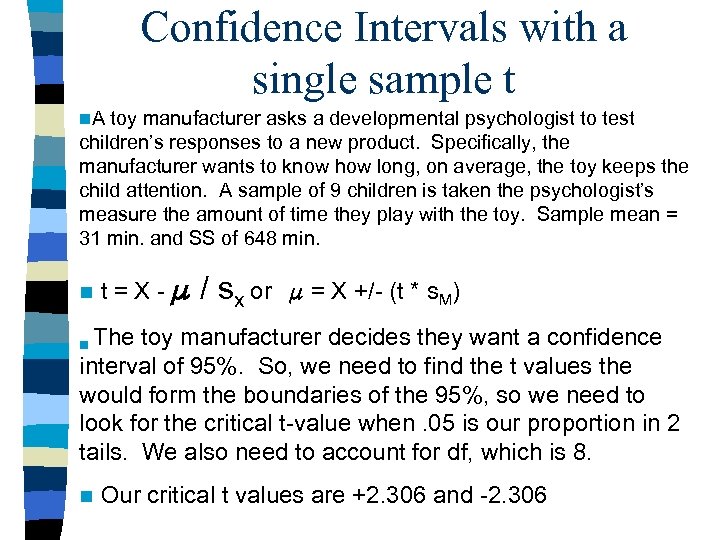Confidence Intervals with a single sample t n. A toy manufacturer asks a developmental psychologist to test children’s responses to a new product. Specifically, the manufacturer wants to know how long, on average, the toy keeps the child attention. A sample of 9 children is taken the psychologist’s measure the amount of time they play with the toy. Sample mean = 31 min. and SS of 648 min. n t=X- / sx or = X +/- (t * s. M) The toy manufacturer decides they want a confidence interval of 95%. So, we need to find the t values the would form the boundaries of the 95%, so we need to look for the critical t-value when. 05 is our proportion in 2 tails. We also need to account for df, which is 8. n n Our critical t values are +2. 306 and -2. 306

Confidence Intervals with a single sample t n. A toy manufacturer asks a developmental psychologist to test children’s responses to a new product. Specifically, the manufacturer wants to know how long, on average, the toy keeps the child attention. A sample of 9 children is taken the psychologist’s measure the amount of time they play with the toy. Sample mean = 31 min. and SS of 648 min. n t=X- n. Our n / sx or = X +/- (t * s. M) critical t values are 2. 306 and -2. 306 Estimate the range of our population mean 2. 3 = 31 - / 6. 9 = 31 - = 24. 2 3 -2. 3 = 31 - / -6. 9 = 31 - = 37. 9 3

Let’s Try One n You want to know how many times on average college students order pizza a month. You take a sample of 25 college students and find that they on average ordered pizza 1. 8 times per week with a SS of 326. n Do a point estimate n Calculate a confidence interval of 90%

Independent-Measures n 1 - 2 = (M 1 - M 2) +/- ts(M-M) n Let’s compute a point estimate and a confidence interval using 95% confidence interval Sample 1 n = 10 M = 25 SS = 250 Sample 2 n=5 M = 33 SS = 140 t= (M 1 - M 2) - ( 1 - 2) s. M 1 - M 2

Repeated Measures n D = MD +/- ts. M n Let’s compute a point estimate and a confidence interval using 90% confidence interval MD = 21 n SS = 1215 n n = 15 n D t= MD - D s. M

Factors affect CI width n To gain more confidence in your estimate you must increase the width n The larger the level of confidence (%) the larger the t value and the larger the interval n Interval width decrease as n increases – Bigger sample gives more info about the population, so we can make a more precise estimate – Sample size controls the magnitude of standard error

Homework n Chapter 11: – 1, 2, 3, 7, 9, 10, 11 n Chapter 12: – 1, 3, 5, 6, 9, 10, 12