Lecture 7 Key issues Consumption depends

Lecture 7 • Key issues • Consumption depends on current income as well as expected future income and wealth • Investment depends on current and expected profits as well as current and expected real interest rates • Investment is the most volatile component of aggregate demand (comprising C + I + G)

Structure of Lecture 1. Overview 2. Consumption 3. Investment 4. The volatility of consumption and investment

1. Overview • Consumption and Investment are important components of the private sector’s demand for output (Y = C + I + G + X - M) • Consumption typically accounts for the largest portion of the GDP – In the US household consumption accounts for about 70% of GDP in the US – In SA household consumption accounted for over 65% of the GDP • Investment – In SA investment levels have stagnated from a high level of just under 30% of GDP in the 1970’s to around 16% of GDP in the early 2000’s to just under 20% of GDP currently – Government’s has set a target to lift investment to 25% of GDP

Keynes consumption function: C = a + b. Yd “The fundamental psychological law upon which we are entitled to depend with great confidence both a priori from our knowledge of human nature and from the detailed facts of experience, is that men are disposed as a rule and on the average, to increase their consumption as their income increases, but not by as much as the increase in their incomes” - JM Keynes “The General Theory of Employment, Interest and Money” (1936)

Implication: APC declines as Y rises Average Propensity to Consume (APC) is given by C/Yd and has the following properties: 1. Consumption is not a constant fraction of disposable income (not a proportional relationship between C and Y) 2. APC declines as Yd increases (indicating that as Yd rises households consume a smaller fraction of output and their savings increase as a fraction of Yd) (Keynesian regarded this property as fundamental to his view that government policy interventions would be needed maintain sufficient demand in the economy – The two reasons for Keynes why government demand manageme is necessary to manage inherently volatile AD: 1. The tendency for a decline in APC as Y increases (and higher savings do not transform into investment 2. And the uncertainty faced by investors particularly resulting in investment volatility

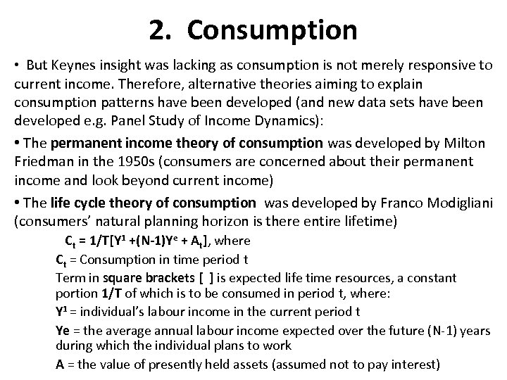2. Consumption • But Keynes insight was lacking as consumption is not merely responsive to current income. Therefore, alternative theories aiming to explain consumption patterns have been developed (and new data sets have been developed e. g. Panel Study of Income Dynamics): • The permanent income theory of consumption was developed by Milton Friedman in the 1950 s (consumers are concerned about their permanent income and look beyond current income) • The life cycle theory of consumption was developed by Franco Modigliani (consumers’ natural planning horizon is there entire lifetime) Ct = 1/T[Y 1 +(N-1)Ye + At], where Ct = Consumption in time period t Term in square brackets [ ] is expected life time resources, a constant portion 1/T of which is to be consumed in period t, where: Y 1 = individual’s labour income in the current period t Ye = the average annual labour income expected over the future (N-1) years during which the individual plans to work A = the value of presently held assets (assumed not to pay interest)

Up Close and Personal: Learning from Panel Data Sets Panel data sets are data sets that show the value of one or more variables for many individuals or many firms over time. Among the many questions for which the Panel Study of Income Dynamics (PSID) has been used are: § How much does (food) consumption respond to transitory movements in income—for example, to the loss of income from becoming unemployed? § How much risk sharing is there within families? For example, when a family member becomes sick or unemployed, how much help does he or she get from other family members? § How much do people care about staying geographically close to their families?

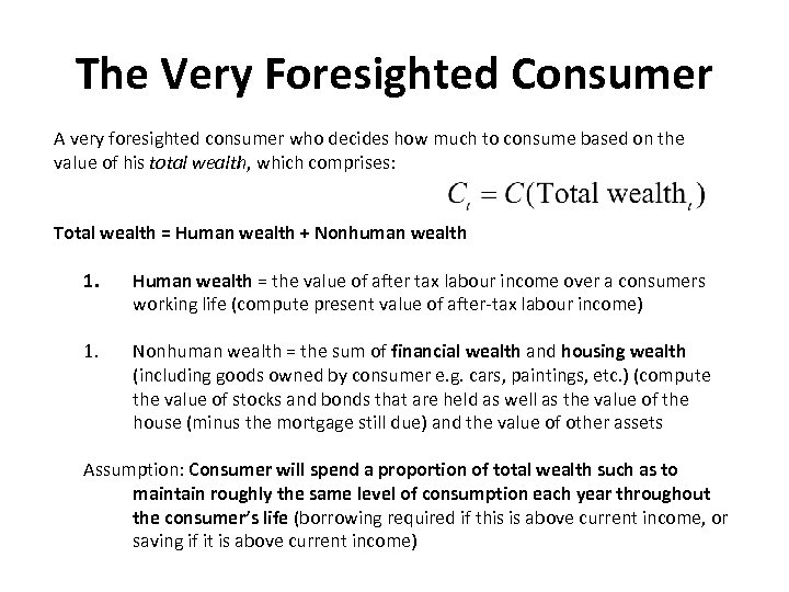The Very Foresighted Consumer A very foresighted consumer who decides how much to consume based on the value of his total wealth, which comprises: Total wealth = Human wealth + Nonhuman wealth 1. Human wealth = the value of after tax labour income over a consumers working life (compute present value of after-tax labour income) 1. Nonhuman wealth = the sum of financial wealth and housing wealth (including goods owned by consumer e. g. cars, paintings, etc. ) (compute the value of stocks and bonds that are held as well as the value of the house (minus the mortgage still due) and the value of other assets Assumption: Consumer will spend a proportion of total wealth such as to maintain roughly the same level of consumption each year throughout the consumer’s life (borrowing required if this is above current income, or saving if it is above current income)

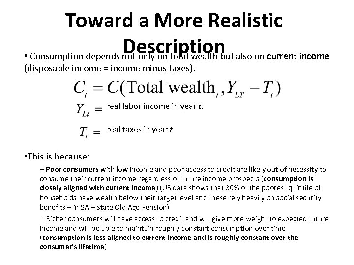Toward a More Realistic Description also on current income • Consumption depends not only on total wealth but (disposable income = income minus taxes). real labor income in year t. real taxes in year t • This is because: – Poor consumers with low income and poor access to credit are likely out of necessity to consume their current income regardless of future income prospects (consumption is closely aligned with current income) (US data shows that 30% of the poorest quintile of households have wealth below their target level and these rely heavily on social security benefits – in SA – State Old Age Pension) – Richer consumers will have access to credit and will give more weight to expected future income and will be able to maintain roughly constant consumption over time (consumption is less aligned to current income and is roughly constant over the consumer’s lifetime)

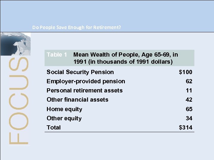Do People Save Enough for Retirement? Table 1 Mean Wealth of People, Age 65 -69, in 1991 (in thousands of 1991 dollars) Social Security Pension $100 Employer-provided pension 62 Personal retirement assets 11 Other financial assets 42 Home equity 65 Other equity 34 Total $314

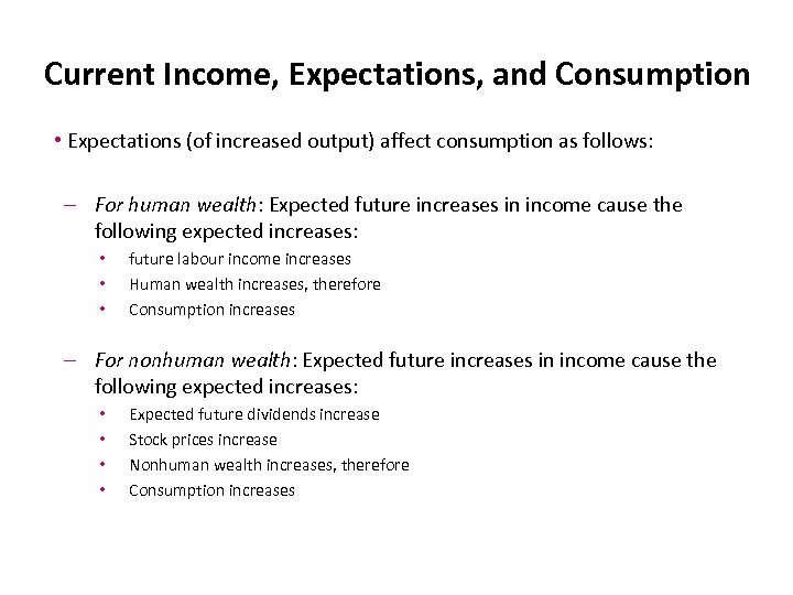Current Income, Expectations, and Consumption • Expectations (of increased output) affect consumption as follows: – For human wealth: Expected future increases in income cause the following expected increases: • • • future labour income increases Human wealth increases, therefore Consumption increases – For nonhuman wealth: Expected future increases in income cause the following expected increases: • • Expected future dividends increase Stock prices increase Nonhuman wealth increases, therefore Consumption increases

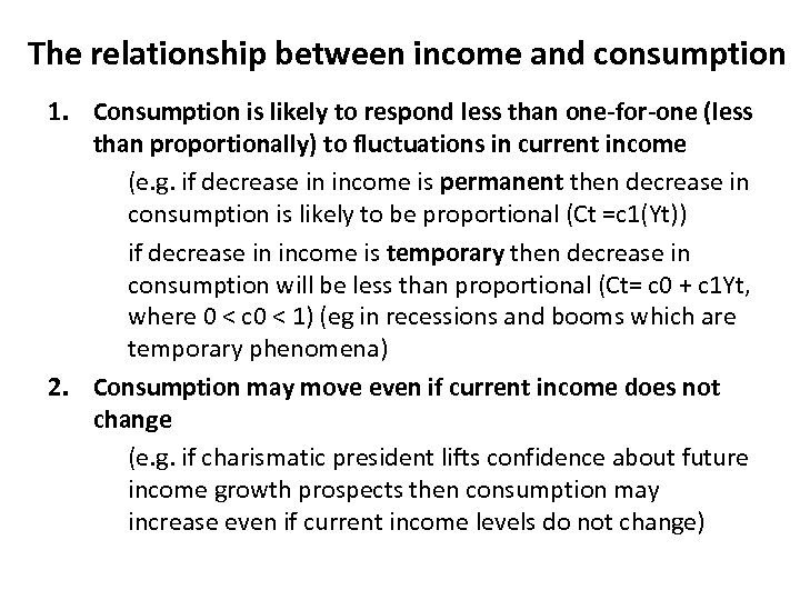The relationship between income and consumption 1. Consumption is likely to respond less than one-for-one (less than proportionally) to fluctuations in current income (e. g. if decrease in income is permanent then decrease in consumption is likely to be proportional (Ct =c 1(Yt)) if decrease in income is temporary then decrease in consumption will be less than proportional (Ct= c 0 + c 1 Yt, where 0 < c 0 < 1) (eg in recessions and booms which are temporary phenomena) 2. Consumption may move even if current income does not change (e. g. if charismatic president lifts confidence about future income growth prospects then consumption may increase even if current income levels do not change)

3. Investment • Investment decisions depend on current sales, the current real interest rate, and on expectations of the future. • The decision to buy a machine depends on the present value of the profits the firm can expect from having this machine versus the cost of buying it. • How do we calculate the present value of expected profits? (first let’s look at the impact of capital depreciation)

Investment and Expectations of Profit • The depreciation rate, , measures how much usefulness the machine from one year to the next. • A machine that is new this year is worth only (1 - ) next year and (1 - )2 in two years time, etc. • Reasonable values for are between 4% and 15% for machines, and between 2% and 4% for buildings and factories.

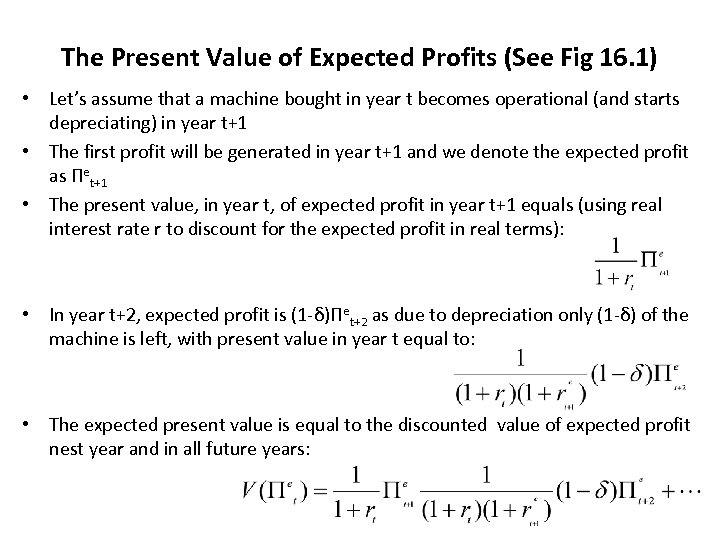The Present Value of Expected Profits (See Fig 16. 1) • Let’s assume that a machine bought in year t becomes operational (and starts depreciating) in year t+1 • The first profit will be generated in year t+1 and we denote the expected profit as Πet+1 • The present value, in year t, of expected profit in year t+1 equals (using real interest rate r to discount for the expected profit in real terms): • In year t+2, expected profit is (1 -δ)Πet+2 as due to depreciation only (1 -δ) of the machine is left, with present value in year t equal to: • The expected present value is equal to the discounted value of expected profit nest year and in all future years:

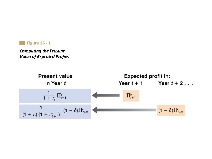Figure 16 - 1 Computing the Present Value of Expected Profits

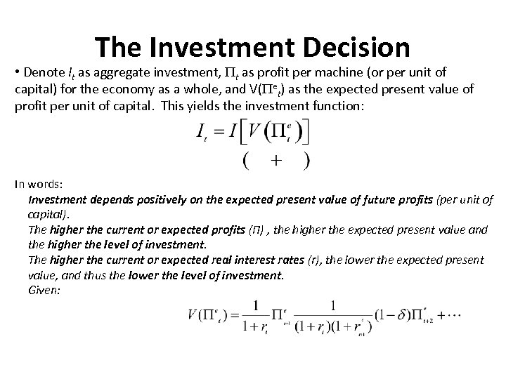The Investment Decision • Denote It as aggregate investment, t as profit per machine (or per unit of capital) for the economy as a whole, and V( et) as the expected present value of profit per unit of capital. This yields the investment function: In words: Investment depends positively on the expected present value of future profits (per unit of capital). The higher the current or expected profits (Π) , the higher the expected present value and the higher the level of investment. The higher the current or expected real interest rates (r), the lower the expected present value, and thus the lower the level of investment. Given:

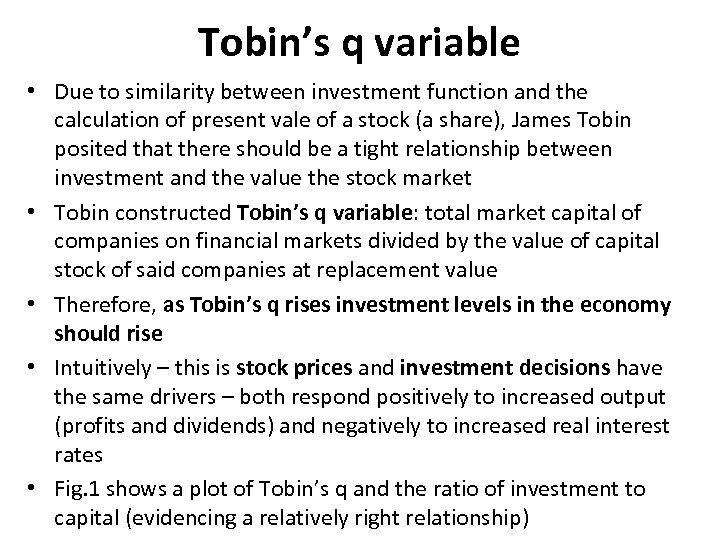Tobin’s q variable • Due to similarity between investment function and the calculation of present vale of a stock (a share), James Tobin posited that there should be a tight relationship between investment and the value the stock market • Tobin constructed Tobin’s q variable: total market capital of companies on financial markets divided by the value of capital stock of said companies at replacement value • Therefore, as Tobin’s q rises investment levels in the economy should rise • Intuitively – this is stock prices and investment decisions have the same drivers – both respond positively to increased output (profits and dividends) and negatively to increased real interest rates • Fig. 1 shows a plot of Tobin’s q and the ratio of investment to capital (evidencing a relatively right relationship)

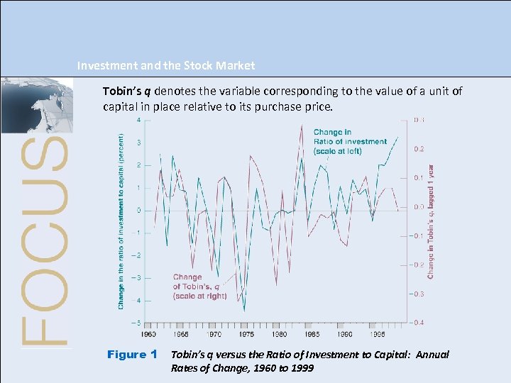Investment and the Stock Market Tobin’s q denotes the variable corresponding to the value of a unit of capital in place relative to its purchase price. Figure 1 Tobin’s q versus the Ratio of Investment to Capital: Annual Rates of Change, 1960 to 1999

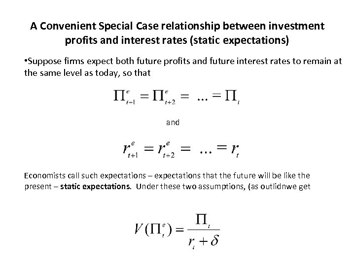A Convenient Special Case relationship between investment profits and interest rates (static expectations) • Suppose firms expect both future profits and future interest rates to remain at the same level as today, so that and Economists call such expectations – expectations that the future will be like the present – static expectations. Under these two assumptions, (as outlidnwe get

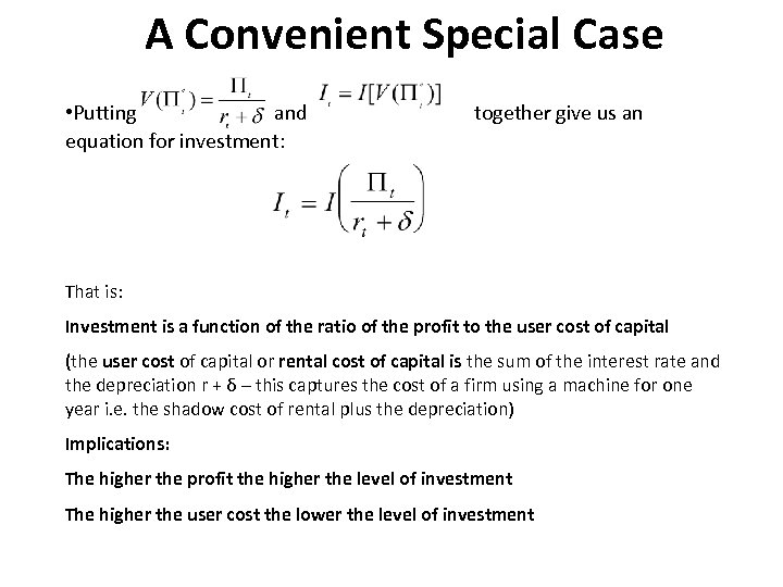A Convenient Special Case • Putting and equation for investment: together give us an That is: Investment is a function of the ratio of the profit to the user cost of capital (the user cost of capital or rental cost of capital is the sum of the interest rate and the depreciation r + δ – this captures the cost of a firm using a machine for one year i. e. the shadow cost of rental plus the depreciation) Implications: The higher the profit the higher the level of investment The higher the user cost the lower the level of investment

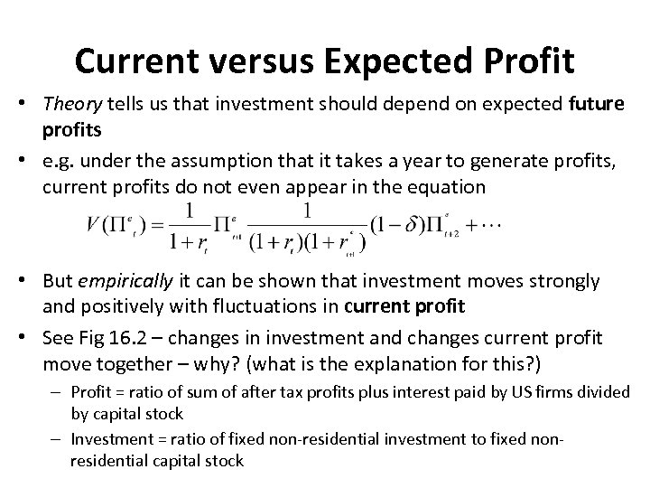Current versus Expected Profit • Theory tells us that investment should depend on expected future profits • e. g. under the assumption that it takes a year to generate profits, current profits do not even appear in the equation • But empirically it can be shown that investment moves strongly and positively with fluctuations in current profit • See Fig 16. 2 – changes in investment and changes current profit move together – why? (what is the explanation for this? ) – Profit = ratio of sum of after tax profits plus interest paid by US firms divided by capital stock – Investment = ratio of fixed non-residential investment to fixed nonresidential capital stock

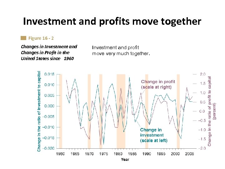Investment and profits move together Figure 16 - 2 Changes in Investment and Changes in Profit in the United States since 1960 Investment and profit move very much together.

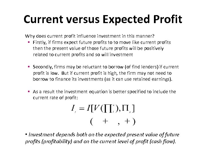Current versus Expected Profit Why does current profit influence investment in this manner? § Firstly, if firms expect future profits to to move like current profits then the present value of those future profits will be positively related to current profits and so will investment § Secondly, firms may be reluctant to borrow (of find lenders) if current profit is low. But if current profit is high, the firm may not need to borrow to finance its investments (as it can use retained earnings). § As a result the investment equation is better specified to include the current rate of profit: • Investment depends both on the expected present value of future profits (profitability) and on the current level of profit (cash flow).

Profitability versus Cash Flow Profitability refers to the expected present discounted value of profits. Cash flow refers to current profit, or the net flow of cash the firm is receiving. Both profitability and cash flow are important for investment decisions, and are likely to move together. Owen Lamont’s undertook a study to prove that cash flow is important to investment. Company A produces steel Company B produces steel and oil (diversified multi-commodity) Where the oil price fell in 1986 company B had reduced cash flows reduced investment in steel (even though still profitable), as compared to company A which continue with its profitable steel investment projects. Note: if for multi-commodity companies the prices of commodities (e. g. oil) are rising this will have a positive effect on cash flow and a positive effect on the investment plans of the company across the multi-commodity spectrum

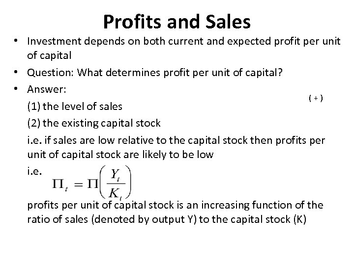Profits and Sales • Investment depends on both current and expected profit per unit of capital • Question: What determines profit per unit of capital? • Answer: (+) (1) the level of sales (2) the existing capital stock i. e. if sales are low relative to the capital stock then profits per unit of capital stock are likely to be low i. e. profits per unit of capital stock is an increasing function of the ratio of sales (denoted by output Y) to the capital stock (K)

Profits and Sales • • • See Fig 16. 3 which plots yearly changes in profit per unit capital (Π) and changes in the ratio of output to capital (Y/K) There is a tight relationship between changes in profit per unit capital (Π) and changes in the ratio of output to capital (Y/K) Given that capital moves slowly over time due to the fact that the stock of capital is large compared to yearly investment): – most of the changes in profit per unit capital (Π) are due to changes in profit – Most of the changes in the ratio of output to capital (Y/K) come from movements in output Therefore: Profit decreases in recessions (when output is down) and increases in expansions (when output is up) Consequence: current output effects current profit and expected future output affects expected future profit and both current and expected future profits effect investment

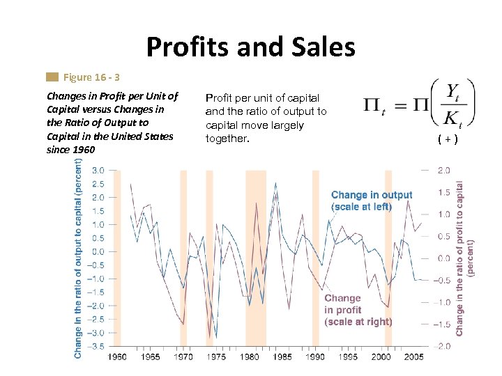Profits and Sales Figure 16 - 3 Changes in Profit per Unit of Capital versus Changes in the Ratio of Output to Capital in the United States since 1960 Profit per unit of capital and the ratio of output to capital move largely together. (+)

4. The Volatility of Consumption and Investment • There are similarities and differences in consumption and investment behaviour: • Similarities – Whether consumers perceive current movements in income to be transitory or permanent affects their consumption decisions. – In the same way, whether firms perceive current movements in sales to be transitory or permanent affects their investment decisions. (e. g. seasonal booms in sales around Christmas do not lead to a boom in investment every year in December)

The Volatility of Consumption and Investment • Differences between consumption decisions and investment decisions: – When faced with an increase in income that consumers perceive as permanent, they respond with at most an equal increase in consumption. They will not increase consumption more than one-for-one with an increase in income as this will require them to cut consumption later – When firms are faced with an increase in sales they believe to be permanent, their present value of expected profits increases, leading to an increase in investment. The increase in investment may be larger than one-for-one as compared to the increase in sales (output) i. e. the increase in sales mat result in a quick, large short-lived increase in investment spending (hence greater volatility)

Investment is more volatile than consumption • See Fig 16. 4 which plots yearly rates of change in US consumption and investment since 1960 (plotted as deviations from the average rate of change) • The figure yields three conclusions: § Consumption and investment usually move together (both C and I decrease during recessions when current income is down). § Investment is much more volatile than consumption i. e the relative movements of I range from -16% to 12%, for C from -4% to 3%. § Because, however, the value of investment is much smaller than the consumption (16% of GDP v 70% of GPD in US), changes in the magnitude of investment from one year to the next end up being of a similar overall magnitude to changes in consumption.

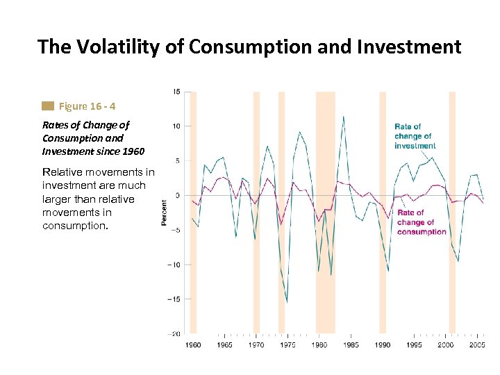The Volatility of Consumption and Investment Figure 16 - 4 Rates of Change of Consumption and Investment since 1960 Relative movements in investment are much larger than relative movements in consumption.