Lecture 5 Consumption&Savings Lecture 5: Consumption

Lecture 5 Consumption&Savings

Lecture 5: Consumption & Savings 1. Consumption Function 2. Saving Function 3. The Paradox of Thrift and The Keynesian Cross

Lecture 5: Consumption & Savings Marginal Propensity to Consume – гранична схильність до споживання Average Propensity to Consume – середня схильність до споживання Marginal Propensity to Save – гранична схильність до заощадження Average Propensity to Save – середня схильність до заощадження The Paradox of Thrift – парадокс заощадження

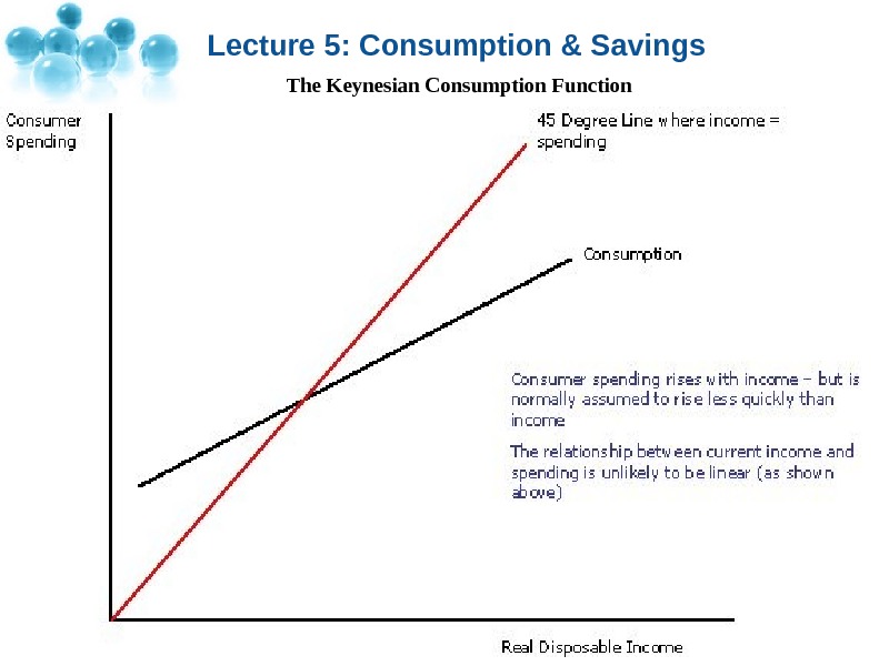
Lecture 5: Consumption & Savings The consumption function isasinglemathematicalfunctionused toexpress consumer spending. Itwasdevelopedby John Maynard Keynes anddetailedmostfamouslyinhisbook The General Theory of Employment, Interest, and Money. Itcapturesthefundamentalpsychologicallawputforthby. Keynes that consumption expenditures by the household sector depend on income and than only a portion of additional income is used for consumption. Thisisexplainedbythefactthat disposableincomeisdividedon consumption and savings and thegrowthofdisposableincomeincreasesconsumptionand savings. Yd = C + S

Lecture 5: Consumption & Savings The function is used to calculate the amount of total consumption in an economy. It is made up of autonomous consumption that is not influenced by current income and induced consumption that is influenced by the economy’s income level. The simple consumption function is shown as the linear function: C = c + mpc*Y where: C – total consumption, c – autonomous consumption (c > 0), mpc – the marginal propensity to consume (ie the induced consumption) (0 < mpc < 1), Y – disposable income (income after taxes and transfer payments, or W – T). 0 d d

Lecture 5: Consumption & Savings Autonomous consumption (also exogenous consumption ) is a term used to describe consumption expenditure that occurs when income levels are zero. Such consumption is considered autonomous of income only when expenditure on these consumables does not vary with changes in income. If income levels are actually zero, this consumption counts as dissaving, because it is financed by borrowing or using up savings. Induced consumption describes consumption expenditure by households on goods and services which varies with income. Such consumption is considered induced by income when expenditure on these consumables varies as income changes.

Lecture 5: Consumption & Savings The Keynesian Consumption Function

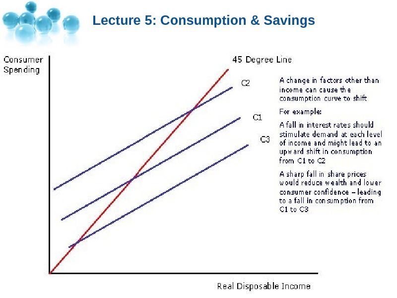
Lecture 5: Consumption & Savings A Shift in the Consumption Function The consumption-income relationship changes when other factors than income change — for example a rise in interest rates or a fall in consumer confidence might lead to a fall in consumption spending at each level of income. A rise in household wealth or a rise in consumer’s expectations might lead to an increased level of consumer demand at each income level (an upward shift in the consumption curve).

Lecture 5: Consumption & Savings

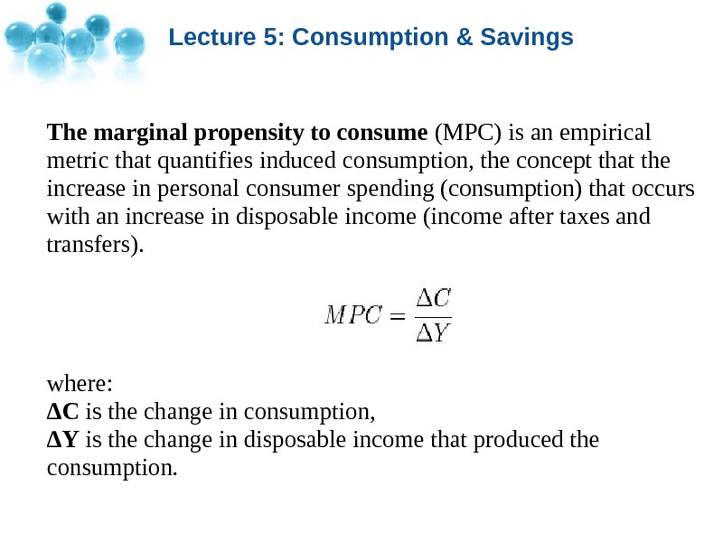
Lecture 5: Consumption & Savings The marginal propensity to consume (MPC) is an empirical metric that quantifies induced consumption, the concept that the increase in personal consumer spending (consumption) that occurs with an increase in disposable income (income after taxes and transfers). where: ΔC is the change in consumption, ΔY is the change in disposable income that produced the consumption.

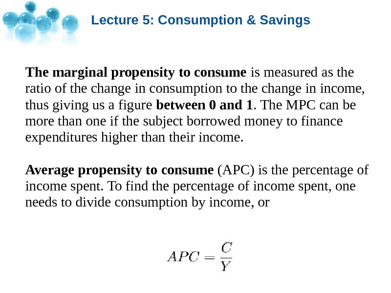
Lecture 5: Consumption & Savings The marginal propensity to consume is measured as the ratio of the change in consumption to the change in income, thus giving us a figure between 0 and 1. The MPC can be more than one if the subject borrowed money to finance expenditures higher than their income. Average propensity to consume (APC) is the percentage of income spent. To find the percentage of income spent, one needs to divide consumption by income, or

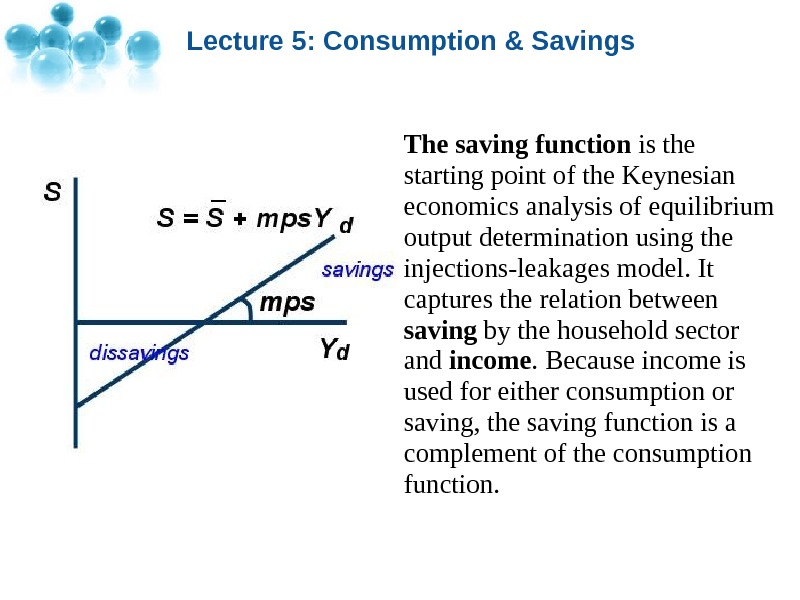
Lecture 5: Consumption & Savings The saving function is the starting point of the Keynesian economics analysis of equilibrium output determination using the injections-leakages model. It captures the relation between saving by the household sector and income. Because income is used for either consumption or saving, the saving function is a complement of the consumption function.

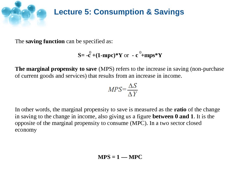
Lecture 5: Consumption & Savings The saving function can be specified as: S= -c +(1 -mpc)*Y or — c +mps*Y The marginal propensity to save (MPS) refers to the increase in saving (non-purchase of current goods and services) that results from an increase in income. In other words, the marginal propensity to save is measured as the ratio of the change in saving to the change in income, also giving us a figure between 0 and 1. It is the opposite of the marginal propensity to consume (MPC). In a two sector closed economy MPS = 1 — MP

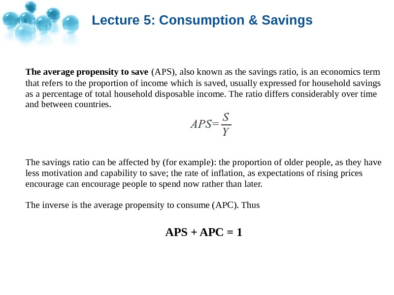
Lecture 5: Consumption & Savings The average propensity to save (APS), also known as the savings ratio, is an economics term that refers to the proportion of income which is saved, usually expressed for household savings as a percentage of total household disposable income. The ratio differs considerably over time and between countries. The savings ratio can be affected by (for example): the proportion of older people, as they have less motivation and capability to save; the rate of inflation, as expectations of rising prices encourage can encourage people to spend now rather than later. The inverse is the average propensity to consume (APC). Thus APS + APC =

Lecture 5: Consumption & Savings Because spending and saving are two sides of the same decision, saving is affected by the same determinants that affect consumption. Here a few of the more important ones: — Interest Rates — Consumer Confidence — Physical Wealth — Financial Wealth — Inflationary Expectations

Lecture 5: Consumption & Savings The paradox of thrift (or paradox of saving ) is a paradox of economics, popularized by John Maynard Keynes. The paradox states that if everyone tries to save more money during times of recession, then aggregate demand will fall and will in turn lower total savings in the population because of the decrease in consumption and economic growth. This paradox can be explained by analyzing the place, and impact, of increased savings in an economy. If a population saves more money (that is the marginal propensity to save increases across all income levels), then total revenues for companies will decline. This decrease in economic growth means fewer salary increases and perhaps downsizing. Eventually the population’s total savings will have remained the same or even declined because of lower incomes and a weaker economy. This paradox is based on the proposition, put forth in Keynesian economics, that many economic downturns are demand based.

Lecture 5: Consumption & Savings In the Keynesian cross diagram (or 45 -degree line diagram), a desired total spending (or aggregate expenditure , or «aggregate demand») curve is drawn as a rising line since consumers will have a larger demand with a rise in disposable income, which increases with total national output. This increase is due to the positive relationship between consumption and consumers disposable income in the consumption function.

Finally.