Lecture 4 Themes in this session Data mining

Lecture 4 Themes in this session Data mining Decision support models Reading Requirements [EN] chapter 26 (second half) G. p. Huber, The Nature of Organizational Decision Making and Design of Decision Support Systems

What is data mining? “Data Mining is data analysis in order to discover hidden correlations (pattern, rules) in huge data sets” “Data Mining is the process of extracting valid, previously unknown, comprehensible, and actionable information from large databases and using it to make crucial business decisions. ”

What is KDD? • Knowledge Discovery in Databases involves the extraction of implicit, previously unknown and potentially useful information from data.

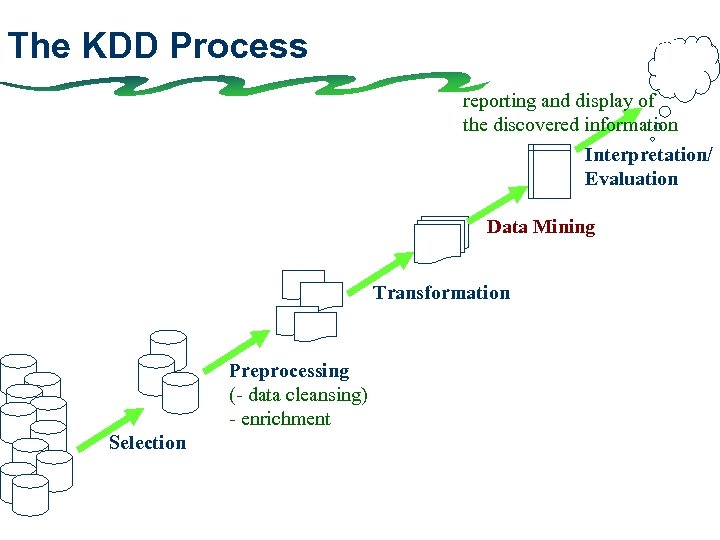The KDD Process Knowledge reporting and display of the discovered information Patterns Transformed data Target Data Preprocessed Data Mining Transformation Data Preprocessing (- data cleansing) - enrichment Selection Interpretation/ Evaluation

Enabling factors for data mining Data availability • Increased amount of electronically stored data • Increased processing power • Increased data storage ability • Increased data gathering ability (networks, extraction tools) • Increased number of data warehouses Business conditions • Increased need to compete effectively • Increased awareness of need to know customers

Data mining uses in enterprises • Predict customer pattern of behaviour, e. g buying pattern • Discover market developments driven by demographic changes • Discover shifts in consumption • Identification of new customers • Anticipation of demands on inventory

Goals of data mining and KD • Prediction data mining can show certain attributes within the data may behave in the future • Identification data patterns can be used to identify the existence of an item, an event, or an activity • Classification data mining can partition the data so that different classes or categories can be identified based on a combination of parameters • Optimisation

Types of KD during data mining • Association rules: the presence of a set of items correlate with another range of values for another set of variables • Classification hierarchies: divide an existing set of events or transaction into a hierarchy of classes • Sequential patterns: detecting association among events with certain temporal relationship • Patterns with time series: position of time series similarities detected within the • Categorisation and segmentation: a given population of events or items can be partitioned (segmented) info sets of “similar” elements

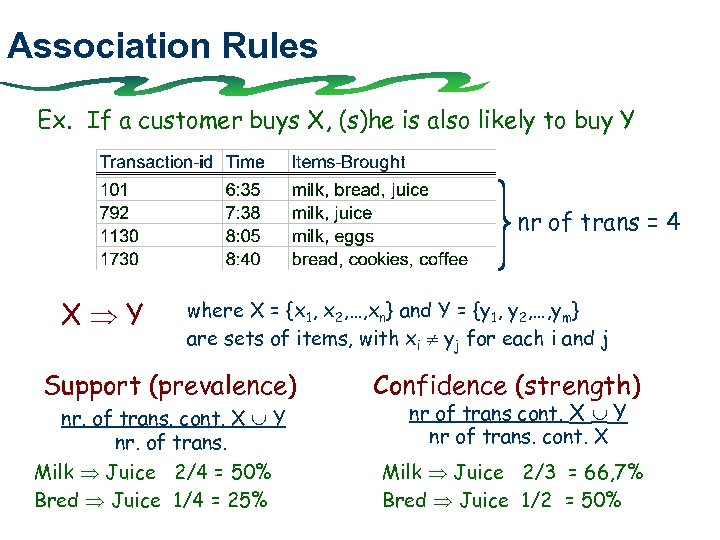Association Rules Ex. If a customer buys X, (s)he is also likely to buy Y nr of trans = 4 X Y where X = {x 1, x 2, …, xn} and Y = {y 1, y 2, …, ym} are sets of items, with xi yj for each i and j Support (prevalence) nr. of trans. cont. X Y nr. of trans. Milk Juice 2/4 = 50% Bred Juice 1/4 = 25% Confidence (strength) nr of trans cont. X Y nr of trans. cont. X Milk Juice 2/3 = 66, 7% Bred Juice 1/2 = 50%

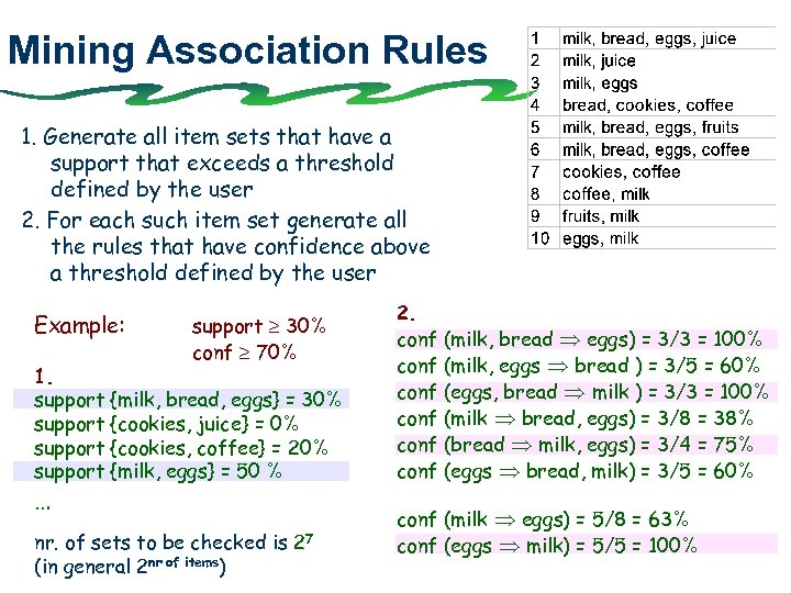Mining Association Rules 1. Generate all item sets that have a support that exceeds a threshold defined by the user 2. For each such item set generate all the rules that have confidence above a threshold defined by the user Example: support 30% conf 70% 1. support {milk, bread, eggs} = 30% support {cookies, juice} = 0% support {cookies, coffee} = 20% support {milk, eggs} = 50 % … nr. of sets to be checked is 27 (in general 2 nr of items) 2. conf conf (milk, bread eggs) = 3/3 = 100% (milk, eggs bread ) = 3/5 = 60% (eggs, bread milk ) = 3/3 = 100% (milk bread, eggs) = 3/8 = 38% (bread milk, eggs) = 3/4 = 75% (eggs bread, milk) = 3/5 = 60% conf (milk eggs) = 5/8 = 63% conf (eggs milk) = 5/5 = 100%

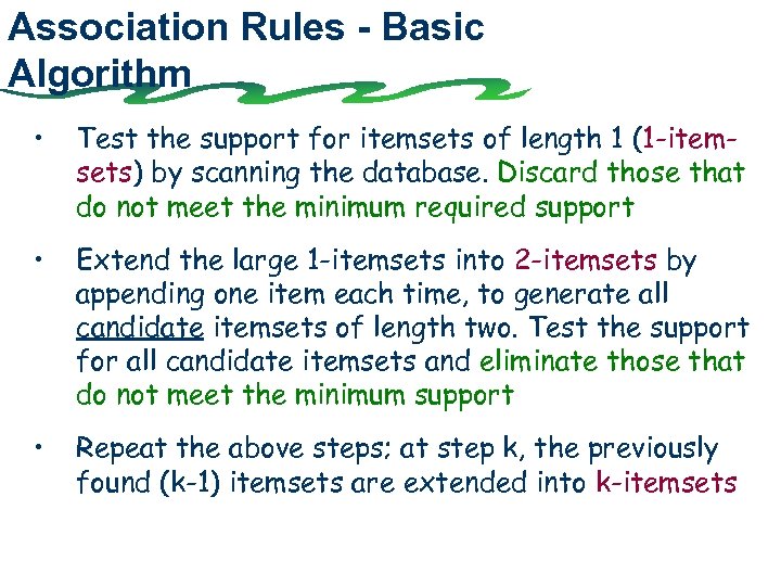Association Rules - Basic Algorithm • Test the support for itemsets of length 1 (1 -itemsets) by scanning the database. Discard those that do not meet the minimum required support • Extend the large 1 -itemsets into 2 -itemsets by appending one item each time, to generate all candidate itemsets of length two. Test the support for all candidate itemsets and eliminate those that do not meet the minimum support • Repeat the above steps; at step k, the previously found (k-1) itemsets are extended into k-itemsets

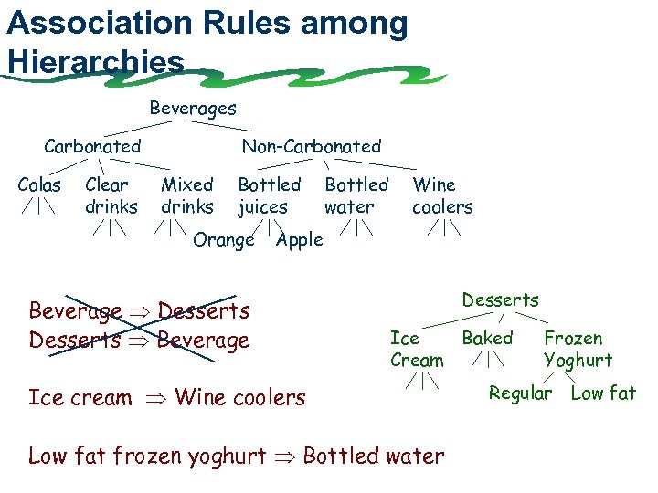Association Rules among Hierarchies Beverages Carbonated Colas Clear drinks Non-Carbonated Mixed drinks Bottled juices Orange Bottled water Wine coolers Apple Beverage Desserts Beverage Desserts Ice Baked Cream Ice cream Wine coolers Low fat frozen yoghurt Bottled water Frozen Yoghurt Regular Low fat

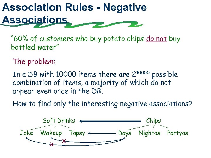Association Rules - Negative Associations “ 60% of customers who buy potato chips do not buy bottled water” The problem: In a DB with 10000 items there are 210000 possible combination of items, a majority of which do not appear even once in the DB. How to find only the interesting negative associations? Soft Drinks Joke Wakeup x x Topsy Chips Days Nightos Partyos

Types of KD during Data Mining • Association rules: the presence of a set of items correlate with another range of values for another set of variables • Classification hierarchies: divide an existing set of events or transaction into a hierarchy of classes • Sequential patterns: detecting association among events with certain temporal relationship • Patterns with time series: position of time series similarities detected within the • Categorisation and segmentation: a given population of events or items can be partitioned (segmented) info sets of “similar” elements

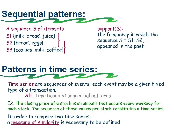Sequential patterns: A sequence S of itemsets S 1 {milk, bread, juice} S 2 {bread, eggs} S 3 {cookies, milk, coffee} support(S): the frequency in which the sequence S = S 1, S 2, . . . appeared in the past Patterns in time series: Time series are sequences of events; each event may be a given fixed type of a transaction. Alt. Time bounded sequential patterns Ex. The closing price of a stock is an amount that occurs every weekday for each stock. The sequence of these values per stock constitutes a time series. In order to compare two time series, a measure of similarity is necessary to be defined.

Types of KD during data mining • Association rules: the presence of a set of items correlate with another range of values for another set of variables • Classification hierarchies: divide an existing set of events or transaction into a hierarchy of classes • Sequential patterns: detecting association among events with certain temporal relationship • Patterns with time series: position of time series similarities detected within the • Categorisation and segmentation: a given population of events or items can be partitioned (segmented) info sets of “similar” elements

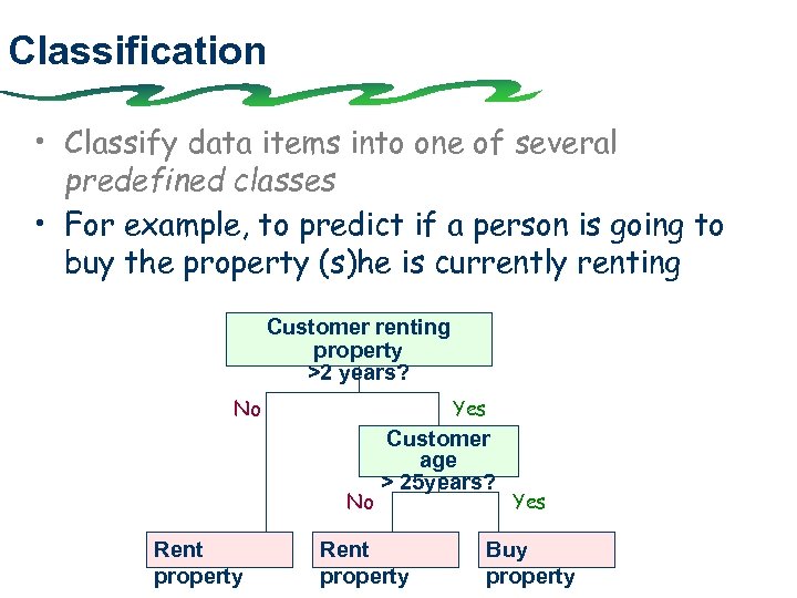Classification • Classify data items into one of several predefined classes • For example, to predict if a person is going to buy the property (s)he is currently renting Customer renting property >2 years? No Yes No Rent property Customer age > 25 years? Rent property Yes Buy property

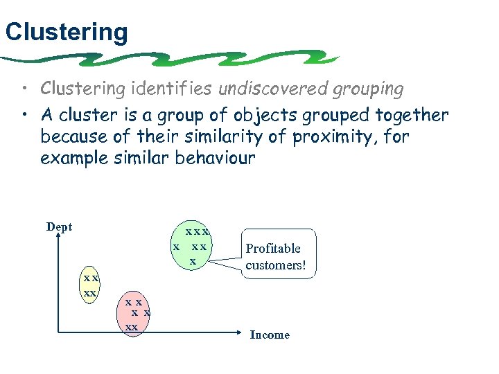Clustering • Clustering identifies undiscovered grouping • A cluster is a group of objects grouped together because of their similarity of proximity, for example similar behaviour Dept XXX X Profitable customers! XX XX X X XX Income

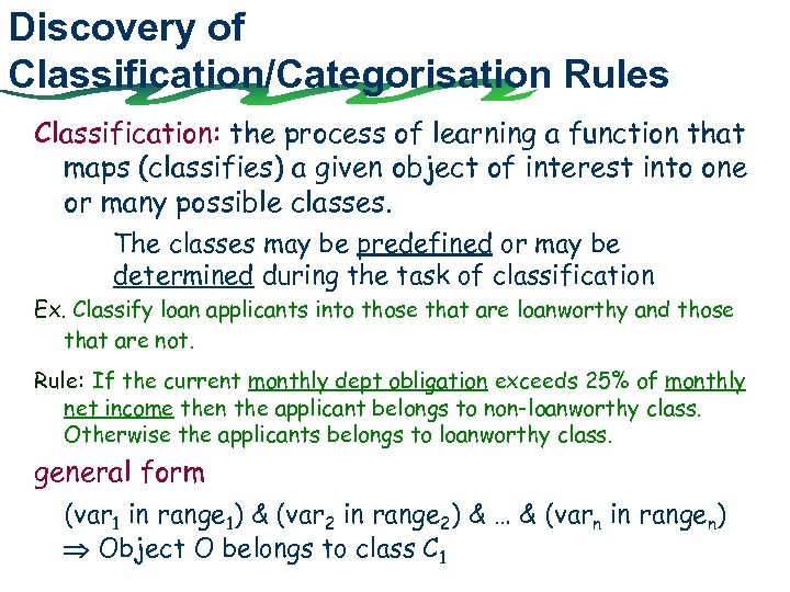Discovery of Classification/Categorisation Rules Classification: the process of learning a function that maps (classifies) a given object of interest into one or many possible classes. The classes may be predefined or may be determined during the task of classification Ex. Classify loan applicants into those that are loanworthy and those that are not. Rule: If the current monthly dept obligation exceeds 25% of monthly net income then the applicant belongs to non-loanworthy class. Otherwise the applicants belongs to loanworthy class. general form (var 1 in range 1) & (var 2 in range 2) & … & (varn in rangen) Object O belongs to class C 1

Data Mining Choosing the function of data mining – includes deciding the purpose of the model derived by the data mining algorithm (e. g. prediction, identification, classification, or optimisation) Choosing the data mining algorithm(s) – includes selecting method(s) to be used for searching for patterns in the data, such as deciding which models and parameters may be appropriate and matching a particular data mining method with the overall criteria of the KDD process

Applications of Data Mining Marketing • analysis of customers behaviour based on buying patterns • determination of marketing strategies including advertising, store location, and targeted mailing • segmentation of customers, stores, or products • design of catalogs, store layouts, and advertising campaigns Finance • analysis of creditworthiness of clients • segmentation of accounts receivables • performance analysis of finance investments like stocks, bonds and mutual funds • evaluation of financing options • fraud detection

Applications of Data Mining 2 Manufacturing • optimisation of resources like machines, manpower and materials • optimal design of manufacturing processes, shop-floor layouts and product design, such as for products tailored according to customers requirements Health Care • analysis of effectiveness of certain treatments • analysis of side effects

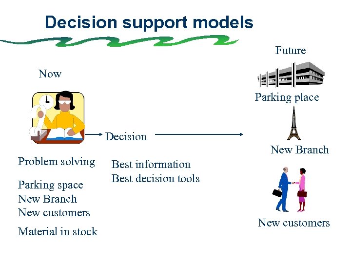Decision support models Future Now Parking place Decision Problem solving Parking space New Branch New customers Material in stock New Branch Best information Best decision tools New customers

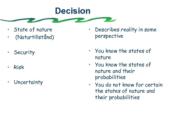Decision • State of nature • (Naturtillstånd) • Describes reality in some perspective • Security • You know the states of nature and their probabilities • You do not know for certain the states of nature and their probabilities • Risk • Uncertainty

Probability • A probability is a number between 0 and 1 which express an relative likelihood for a state of nature to occur • Example: 50 students • marks VG for 15 students, G for 20 students and U for 15 students (or U, 3, 4 and 5) • Probability for VG 15/50=0. 3 • Probability for G 20/50=0. 4 • Probability for U 15/50=0. 3

Expected values Example: Stock portfolios The investor has a choice between three different stock portfolios: I, R, and D and each portfolio gives a different properly discounted, prospective return each year. The yearly return depends upon whether the future brings inflation, recession (lågkonjunktur) or depression

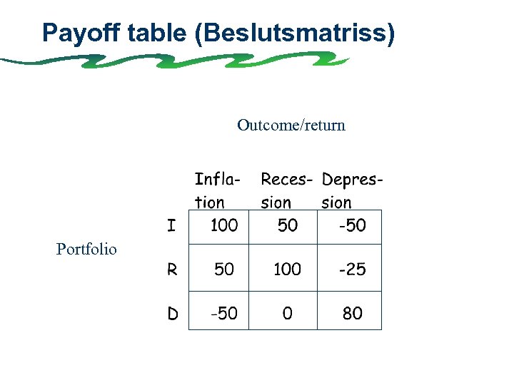Payoff table (Beslutsmatriss) Outcome/return Portfolio

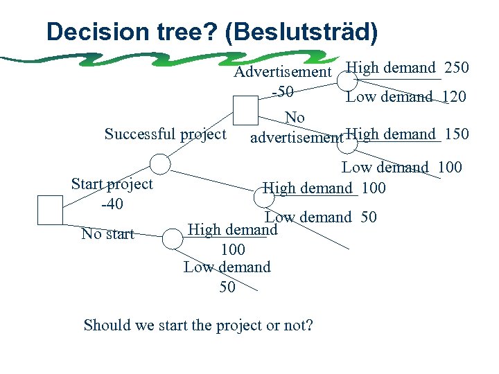Decision tree? (Beslutsträd) Advertisement High demand 250 -50 Low demand 120 No Successful project advertisement High demand 150 Start project -40 No start Low demand 100 High demand 100 Low demand 50 Should we start the project or not?

Decision under risk • Know: The status of nature and their probabilities

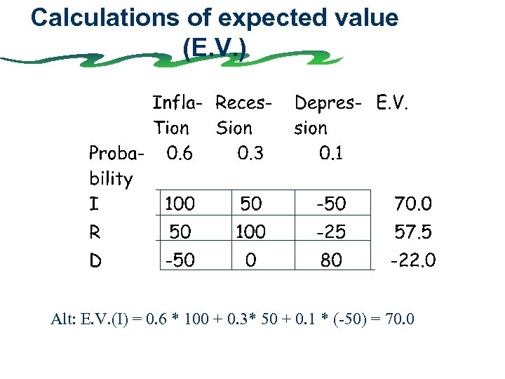Calculations of expected value (E. V. ) Alt: E. V. (I) = 0. 6 * 100 + 0. 3* 50 + 0. 1 * (-50) = 70. 0

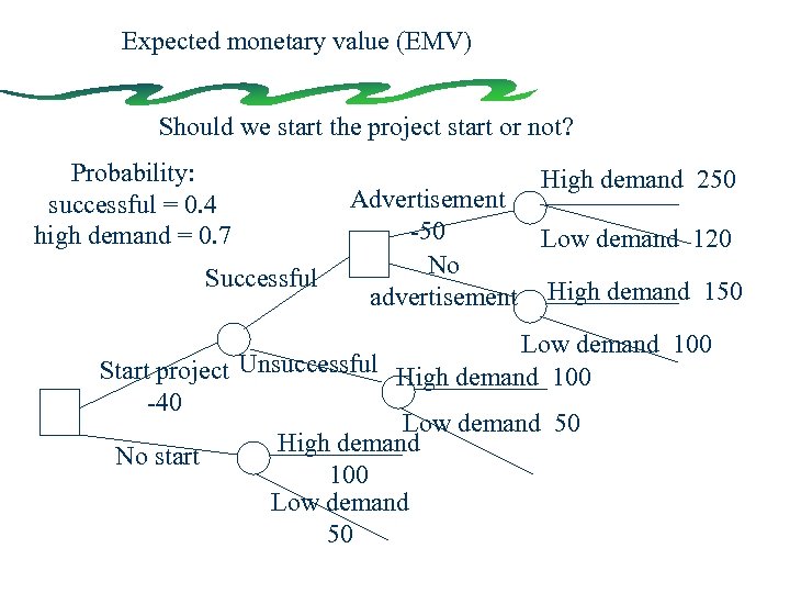Expected monetary value (EMV) Should we start the project start or not? Probability: successful = 0. 4 high demand = 0. 7 Successful High demand 250 Advertisement -50 Low demand 120 No advertisement High demand 150 Low demand 100 Start project Unsuccessful High demand 100 -40 Low demand 50 High demand No start 100 Low demand 50

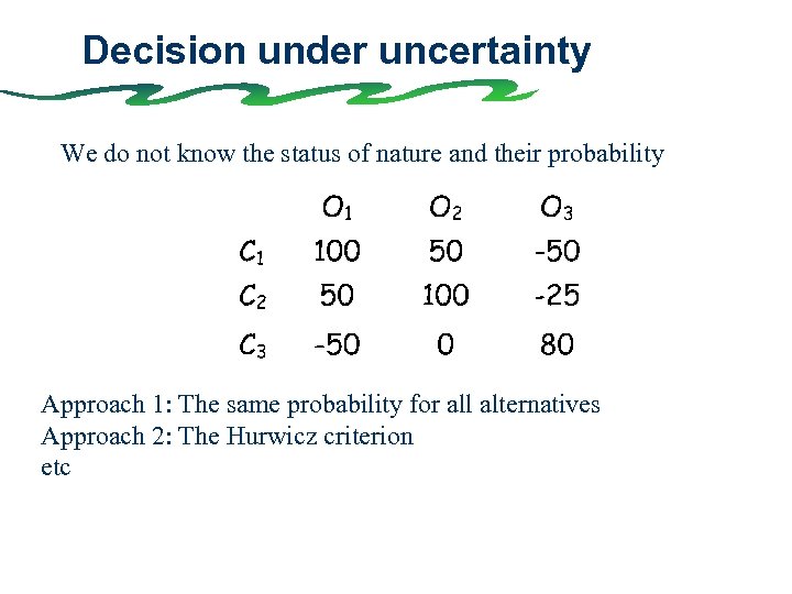Decision under uncertainty We do not know the status of nature and their probability Approach 1: The same probability for all alternatives Approach 2: The Hurwicz criterion etc

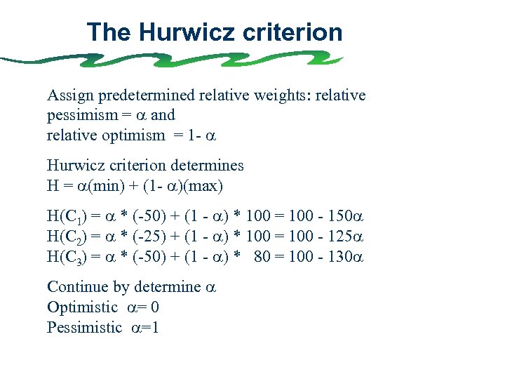The Hurwicz criterion Assign predetermined relative weights: relative pessimism = and relative optimism = 1 - Hurwicz criterion determines H = (min) + (1 - )(max) H(C 1) = * (-50) + (1 - ) * 100 = 100 - 150 H(C 2) = * (-25) + (1 - ) * 100 = 100 - 125 H(C 3) = * (-50) + (1 - ) * 80 = 100 - 130 Continue by determine Optimistic = 0 Pessimistic =1

Linear programming • Narrow down the set of possible alternatives to a set of manageable alternatives • This method can be use to solve problem concerning linear allocation-problems i. g. 6 X + 7 Y = 510 • Optimising • It can be used for choice of – – – products (product combination with max. profit) machinery (min. cost of production) transportation ( min. cost for transportation ) investment (investment combination, with max return)

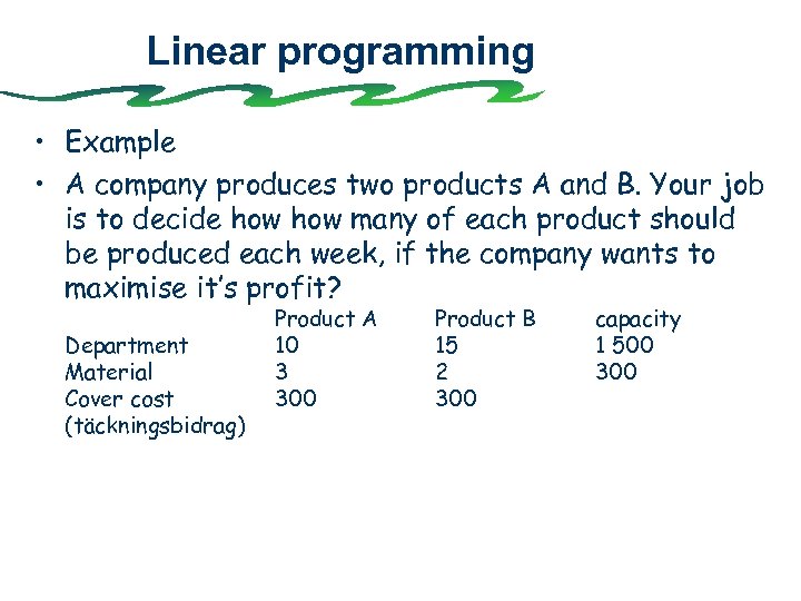Linear programming • Example • A company produces two products A and B. Your job is to decide how many of each product should be produced each week, if the company wants to maximise it’s profit? Department Material Cover cost (täckningsbidrag) Product A 10 3 300 Product B 15 2 300 capacity 1 500 300

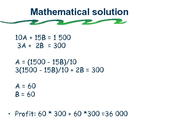Mathematical solution 10 A + 15 B = 1 500 3 A + 2 B = 300 A = (1500 - 15 B)/10 3(1500 - 15 B)/10 + 2 B = 300 A = 60 B = 60 • Profit: 60 * 300 + 60 *300 =36 000

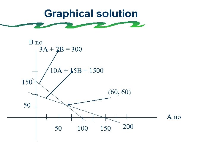Graphical solution B no 3 A + 2 B = 300 10 A + 15 B = 1500 150 (60, 60) 50 A no 50 100 150 200

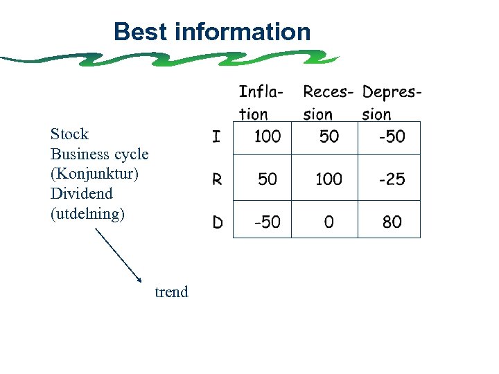Best information Stock Business cycle (Konjunktur) Dividend (utdelning) trend

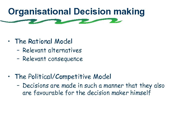Organisational Decision making • The Rational Model – Relevant alternatives – Relevant consequence • The Political/Competitive Model – Decisions are made in such a manner that they also are favourable for the decision maker himself

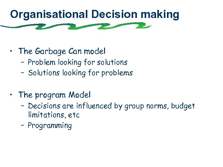Organisational Decision making • The Garbage Can model – Problem looking for solutions – Solutions looking for problems • The program Model – Decisions are influenced by group norms, budget limitations, etc – Programming