Lecture 4 Present or Discounted Value Risk and

Lecture 4 Present (or Discounted) Value, Risk and Return 1. Present (or Discounted) Value 2. Risk and Return 3. Using probability distributions to measure 4. Expected Return and Standard Deviation 5. Risk and return at portfolio context 6. Risk diversification Research work: 1. The main financial indicators of Ukraine and Crimea development for the last 5 years (sources!!!) 2. Financial problems of tourism in Crimea (sources!!!)

Present (or Discounted) Value Calculating the present value of future cash flows allows us to place all cash flows on a current footing so that comparisons can be made in terms of today's dollars

Which should you prefer—$1, 000 today or $2, 000 10 years from today? n n n Assume that both sums are completely certain and your opportunity cost of funds is 8 % per annum The present worth of $1, 000 received today is easy—it is worth $1, 000. What amount (today) would grow to be $2, 000 at the end of 10 years at 8 percent compound interest? This amount is called the present value of $2, 000 payable in 10 years, discounted at 8 percent.

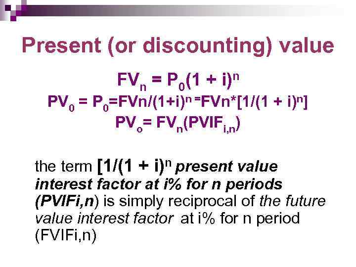Present (or discounting) value FVn = P 0(1 + i)n PV 0 = P 0=FVn/(1+i)n =FVn*[1/(1 + i)n] PVo= FVn(PVIFi, n) the term [1/(1 + i)n present value interest factor at i% for n periods (PVIFi, n) is simply reciprocal of the future value interest factor at i% for n period (FVIFi, n)

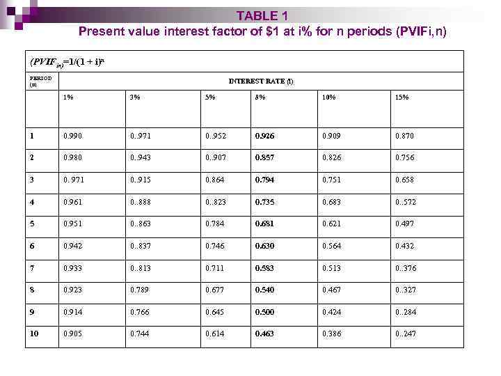TABLE 1 Present value interest factor of $1 at i% for n periods (PVIFi, n) (PVIFin)=1/(1 + i)n PERIOD (n) INTEREST RATE (i) 1% 3% 5% 8% 10% 15% 1 0. 990 0. . 971 0. . 952 0. 926 0. 909 0. 870 2 0. 980 0. . 943 0. . 907 0. 857 0. 826 0. 756 3 0. 971 0. . 915 0. 864 0. 794 0. 751 0. 658 4 0. 961 0. . 888 0. . 823 0. 735 0. 683 0. . 572 5 0. 951 0. . 863 0. 784 0. 681 0. 621 0. 497 6 0. 942 0. . 837 0. 746 0. 630 0. 564 0. 432 7 0. 933 0. . 813 0. 711 0. 583 0. 513 0. . 376 8 0. 923 0. 789 0. 677 0. 540 0. 467 0. . 327 9 0. 914 0. 766 0. 645 0. 500 0. 424 0. . 284 10 0. 905 0. 744 0. 614 0. 463 0. 386 0. . 247

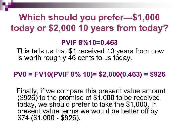Which should you prefer—$1, 000 today or $2, 000 10 years from today? PVIF 8%10=0. 463 This tells us that $1 received 10 years from now is worth roughly 46 cents to us today. PV 0 = FV 10(PVIF 8% 10)= $2, 000(0. 463) = $926 Finally, if we compare this present value amount ($926) to the promise of $1, 000 to be received today, we should prefer to take the $1, 000. In present value terms we would be better off by $74 ($1, 000 - $926).

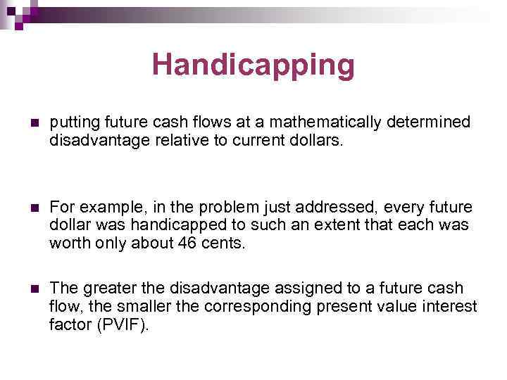Handicapping n putting future cash flows at a mathematically determined disadvantage relative to current dollars. n For example, in the problem just addressed, every future dollar was handicapped to such an extent that each was worth only about 46 cents. n The greater the disadvantage assigned to a future cash flow, the smaller the corresponding present value interest factor (PVIF).

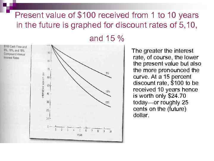Present value of $100 received from 1 to 10 years in the future is graphed for discount rates of 5, 10, and 15 % The greater the interest rate, of course, the lower the present value but also the more pronounced the curve. At a 15 percent discount rate, $100 to be received 10 years hence is worth only $24. 70 today—or roughly 25 cents on the (future) dollar.

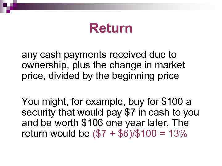Return any cash payments received due to ownership, plus the change in market price, divided by the beginning price You might, for example, buy for $100 a security that would pay $7 in cash to you and be worth $106 one year later. The return would be ($7 + $6)/$100 = 13%

Expected return R= [Dt+(Pt-Pt-1) ]/ Pt-1 R is the actual (expected) return n t refers to a particular time period in the past (future); n Dt is the cash dividend at the end of time period t; n Pt is the stock's price at time period t; and n Pt-1 is the stock's price at time period t -1. n

Risk variability of returns from those that are expected So, T-bill would be a risk-free security while the common stock would be a risky security

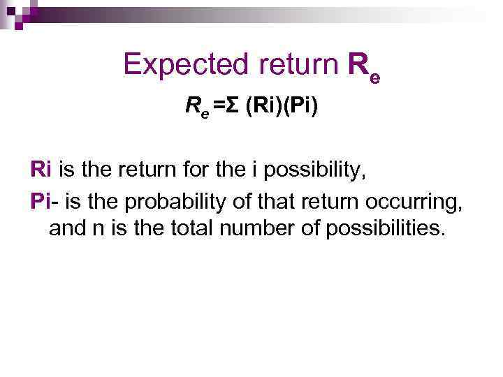Expected return Re Re =Σ (Ri)(Pi) Ri is the return for the i possibility, Pi- is the probability of that return occurring, and n is the total number of possibilities.

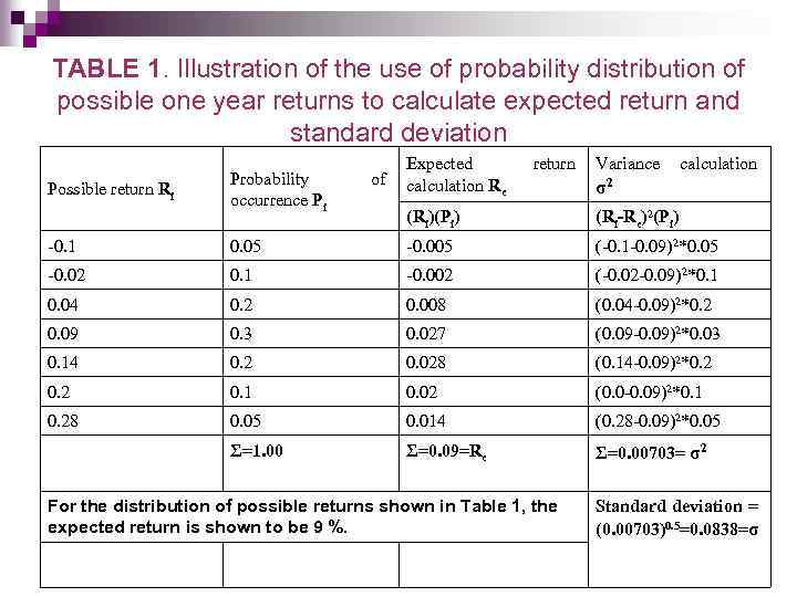TABLE 1. Illustration of the use of probability distribution of possible one year returns to calculate expected return and standard deviation Possible return Ri Probability occurrence Pi of Expected calculation Re return Variance calculation σ2 (Ri)(Pi) (Ri-Re)2(Pi) -0. 1 0. 05 -0. 005 (-0. 1 -0. 09)2*0. 05 -0. 02 0. 1 -0. 002 (-0. 02 -0. 09)2*0. 1 0. 04 0. 2 0. 008 (0. 04 -0. 09)2*0. 2 0. 09 0. 3 0. 027 (0. 09 -0. 09)2*0. 03 0. 14 0. 2 0. 028 (0. 14 -0. 09)2*0. 2 0. 1 0. 02 (0. 0 -0. 09)2*0. 1 0. 28 0. 05 0. 014 (0. 28 -0. 09)2*0. 05 Σ=1. 00 Σ=0. 09=Re Σ=0. 00703= σ2 For the distribution of possible returns shown in Table 1, the expected return is shown to be 9 %. Standard deviation = (0. 00703)0. 5=0. 0838=σ

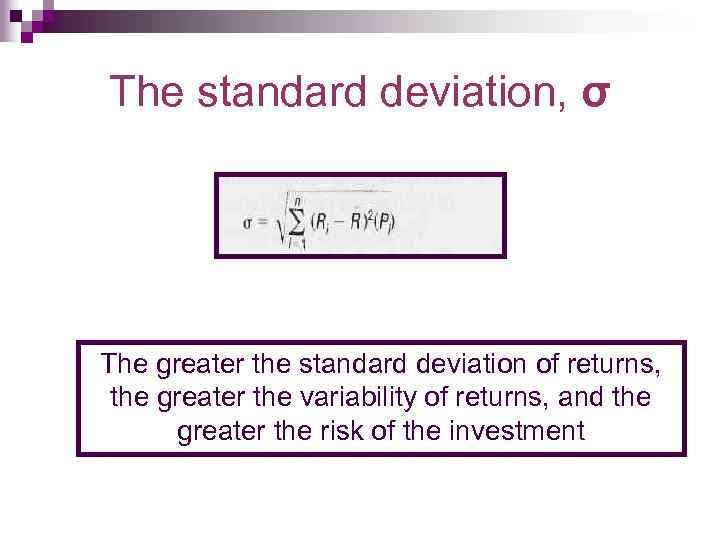The standard deviation, σ The greater the standard deviation of returns, the greater the variability of returns, and the greater the risk of the investment

Variance of the distribution n The square of the standard deviation, σ2 or the weighted average of squared deviations of possible of occurrence n Operationally, we generally first calculate a distribution's variance, or the weighted average of squared deviations of possible of occurrence.

Coefficient of variation (CV) is a measure of relative dispersion (risk)— a measure of risk "per unit of expected return. " The larger the CV, the larger the relative risk of the investment

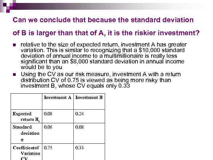Can we conclude that because the standard deviation of В is larger than that of A, it is the riskier investment? n n relative to the size of expected return, investment A has greater variation. This is similar to recognizing that a $10, 000 standard deviation of annual income to a multimillionaire is really less significant than an $8, 000 standard deviation in annual income would be to you Using the CV as our risk measure, investment A with a return distribution CV of 0. 75 is viewed as being more risky than investment B, whose CV equals only 0. 33 Investment A Investment B Expected 0. 08 return Re 0. 24 Standard 0. 06 deviation 0. 08 σ Coefficientof 0. 75 Variation 0. 33

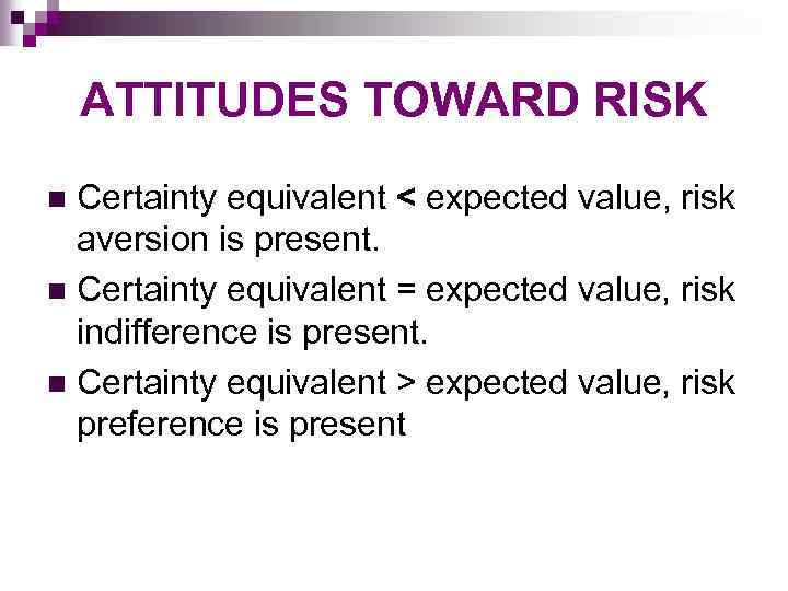ATTITUDES TOWARD RISK Certainty equivalent < expected value, risk aversion is present. n Certainty equivalent = expected value, risk indifference is present. n Certainty equivalent > expected value, risk preference is present n

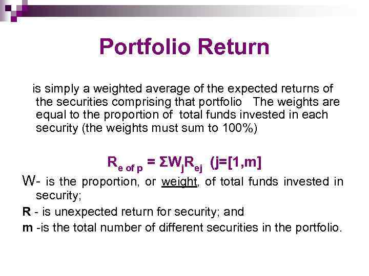Portfolio Return is simply a weighted average of the expected returns of the securities comprising that portfolio The weights are equal to the proportion of total funds invested in each security (the weights must sum to 100%) Re of p = ΣWj. Rej (j=[1, m] W- is the proportion, or weight, of total funds invested in security; R - is unexpected return for security; and m -is the total number of different securities in the portfolio.

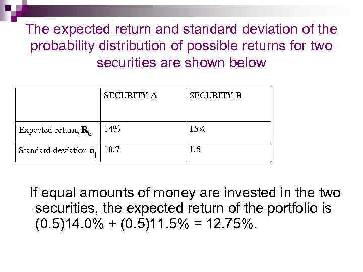The expected return and standard deviation of the probability distribution of possible returns for two securities are shown below SECURITY A Expected return, Re SECURITY В 14% 15% Standard deviation σj 10. 7 1. 5 If equal amounts of money are invested in the two securities, the expected return of the portfolio is (0. 5)14. 0% + (0. 5)11. 5% = 12. 75%.

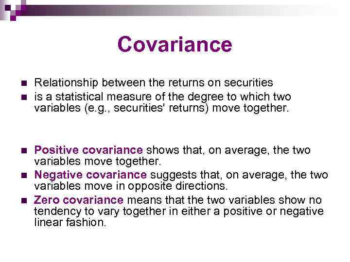Covariance n n n Relationship between the returns on securities is a statistical measure of the degree to which two variables (e. g. , securities' returns) move together. Positive covariance shows that, on average, the two variables move together. Negative covariance suggests that, on average, the two variables move in opposite directions. Zero covariance means that the two variables show no tendency to vary together in either a positive or negative linear fashion.

DIVERSIFICATION n The idea is to spread your risk across a number of assets or investments n It would seem to imply that investing $10, 000 evenly across 10 different securities makes you more diversified than the same amount of money invested evenly across 5 securities. n The catch is that naive diversification ignores the covariance (or correlation) between security returns. The portfolio containing 10 securities could represent stocks from only one industry and have returns that are highly correlated. The 5 -stock portfolio might represent various industries whose security returns might show low correlation and, hence, low portfolio return variability.

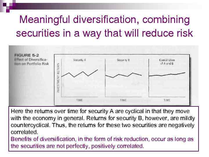Meaningful diversification, combining securities in a way that will reduce risk Here the returns over time for security A are cyclical in that they move with the economy in general. Returns for security B, however, are mildly countercyclical. Thus, the returns for these two securities are negatively correlated. Benefits of diversification, in the form of risk reduction, occur as long as the securities are not perfectly, positively correlated.

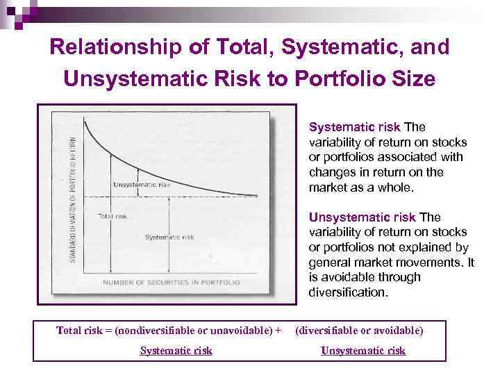Relationship of Total, Systematic, and Unsystematic Risk to Portfolio Size Systematic risk The variability of return on stocks or portfolios associated with changes in return on the market as a whole. Unsystematic risk The variability of return on stocks or portfolios not explained by general market movements. It is avoidable through diversification. Total risk = (nondiversifiable or unavoidable) + Systematic risk (diversifiable or avoidable) Unsystematic risk