Lecture 4 Introductory Econometrics INTRODUCTION TO LINEAR REGRESSION

Lecture 4 Introductory Econometrics INTRODUCTION TO LINEAR REGRESSION MODEL II September 27, 2014

On previous lecture • We studied PRM vs SRM • We listed the classical assumptions of regression models: • • • model linear in parameters, explanatory variables linearly independent (normally distributed) error term with zero mean and constant variance, no serial autocorrelation no correlation between error term and explanatory variables • We saw that if the assumptions hold, OLS estimate is • • consistent unbiased efficient normally distributed

On today’s lecture • We will show that under these assumption, OLS is the best estimator available for regression models • See the distribution, mean and variance of linear regression model parameters • We are going to discuss how hypothesis about coefficients can be tested in regression models • We will explain what significance of coefficients means • We will learn how to read regression output

Distribution of parameters .

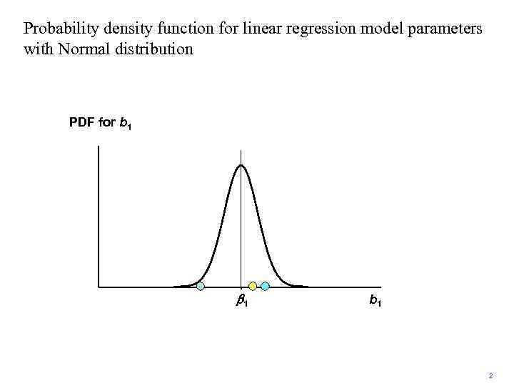Probability density function for linear regression model parameters with Normal distribution PDF for b 1 b 1 2

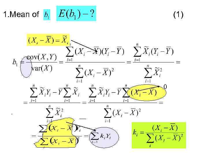1. Mean of (1) 0 .

1. Mean of (2) BLUE -linear estimation random variable . =0 =1 Demonstrate

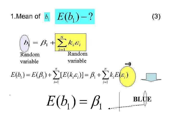1. Mean of Random variable . (3) Random variable =0 BLUE

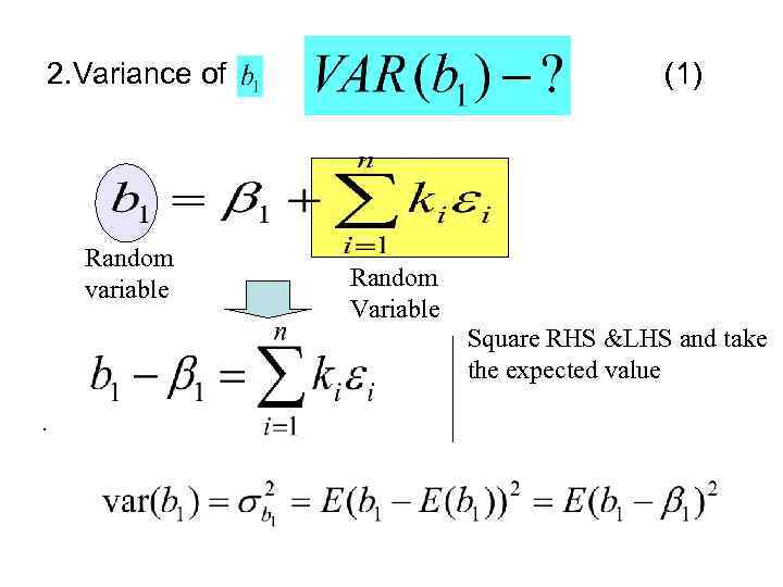2. Variance of Random variable (1) Random Variable Square RHS &LHS and take the expected value .

2. Variance (2) =0.

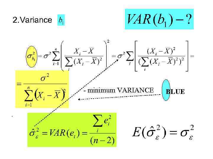2. Variance - minimum VARIANCE. BLUE

Now we will study 1. How to check coefficients for significance 2. Construct confidence intervals for parameters

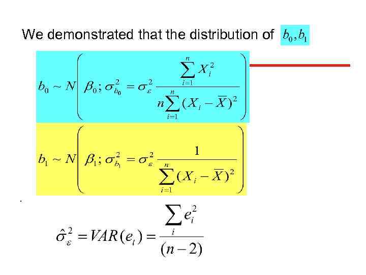We demonstrated that the distribution of .

If are normally distributed, then i=0, 1. k- number of estimated model parameters k=2

PDF for Student’s t-distribution f(t) Region of acceptance Critical or rejection region 0 t Probability of getting into the critical region 2

Significance of the coefficients i=0, 1 Rule: reject null hypothesis H 0 if i=0, 1 . at significance level

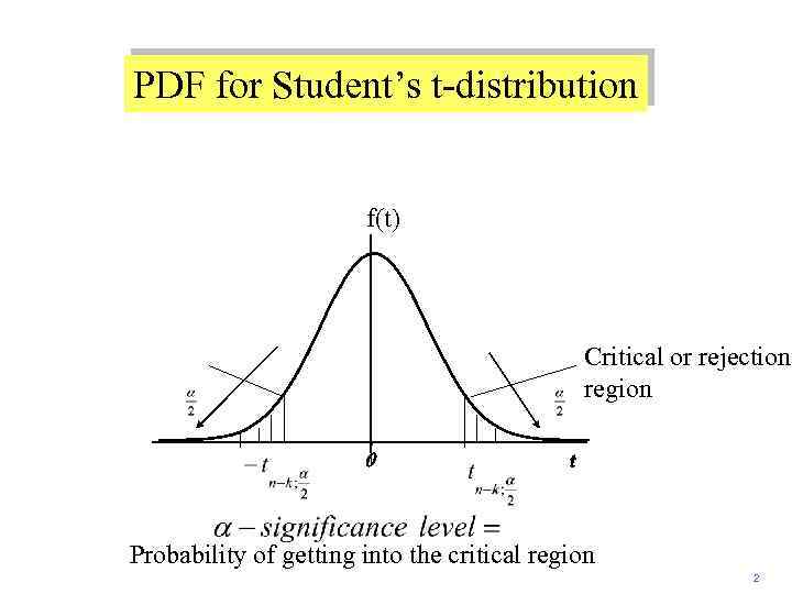PDF for Student’s t-distribution f(t) Critical or rejection region 0 t Probability of getting into the critical region 2

Example from E-Views Real Consumption (CONS 1); Real GDP (GDP 1) Dependent Variable: CONS 1 Method: Least Squares Sample: 2003: 1 2007: 4 Included observations: 16 Variable Coefficient Std. Error t-Statistic Prob. GDP 1 0. 106038 0. 027689 3. 829529 0. 0018 C 4. 695067 0. 814695 5. 762976 0. 0000 R-squared 0. 511604 Mean dependent var 7. 7125 Adjusted R-squared 0. 476719 S. D. dependent var 1. 1451 S. E. of regression 0. 828308 Akaike info criterion 2. 5777 Sum squared resid 9. 605324 Schwarz criterion 2. 6742 F-statistic 14. 666 Prob(F-statistic) 0. 0018 Log likelihood Durbin-Watson stat -18. 62085 1. 061248

Приклад CONS 1 = 4. 7 + 0. 11 GDP 1 (0. 81) s. e. (0. 028) RULE: Reject H 0, if i=0, 1 . with significance level Reject H 0 Conclusion: Intercept is statistically significant

Check for the slope CONS 1 = 4. 7 + 0. 11 GDP 1 (0. 81) . (0. 028) s. e.

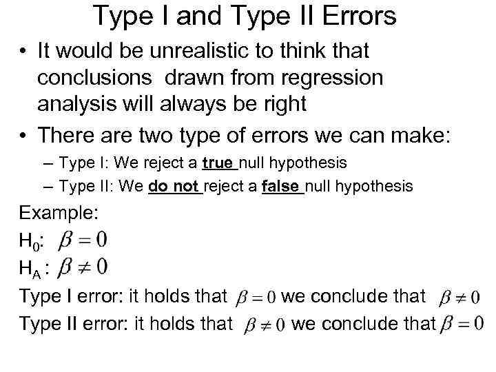Type I and Type II Errors • It would be unrealistic to think that conclusions drawn from regression analysis will always be right • There are two type of errors we can make: – Type I: We reject a true null hypothesis – Type II: We do not reject a false null hypothesis Example: H 0: HA : Type I error: it holds that Type II error: it holds that we conclude that

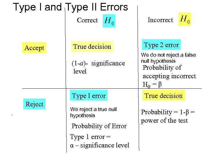Type I and Type II Errors Correct Accept True decision (1 -a)- significance level Type I error Reject. We reject a true null hypothesis Probability of Error Type 1 error = α – significance level Incorrect Type 2 error We do not reject a false null hypothesis Probability of accepting incorrect H 0 = β True decision Probability = 1 -β = power of the test

Type I and Type II Errors Example: • H 0 : The defendant is innocent • HA : The defendant is guilty • Type I error = Sending an innocent person to jail • Type II error = Freeing a guilty person • Obviously, lowering the probability of Type I error means increasing the probability of Type II error • In hypothesis testing, we focus on Type I error and we ensure that its probability is not unreasonably large

Decision Rule • A sample statistic must be calculated that allows the null hypothesis to be rejected or not depending on the magnitude of that sample statistic compared with a preselected critical value found in tables • The critical value divides the range of possible values of the statistic into two regions: acceptance region and rejection region • The idea is that if the value of the coefficient is not such as stated under H 0, the value of the sample statistic should not fall into the rejection region • If the value of the sample statistic falls into the rejection region, we reject H 0

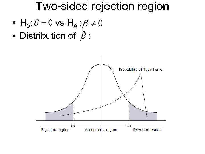Two-sided rejection region • H 0: vs HA : • Distribution of :

P-value Concept (probability value) p-value . -the lowest level of significance at which we reject H 0

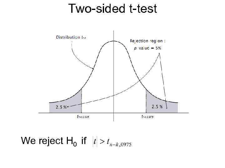Two-sided t-test We reject H 0 if

Example from Stata

Example: P-value for intercept = 0. 000 It means that at any significance level we reject H 0 for intercept, including 10% , 5 % and 1%. . . Conclusion Intercept is statistically significant

Example: i=0, 1 RULE: Reject H 0 , if i=0, 1 At. significance level -significance level is usually given - critical value

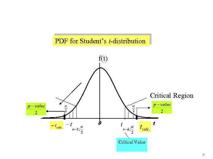PDF for Student’s t-distribution f(t) Critical Region 0 t Critical Value 2

+ . =

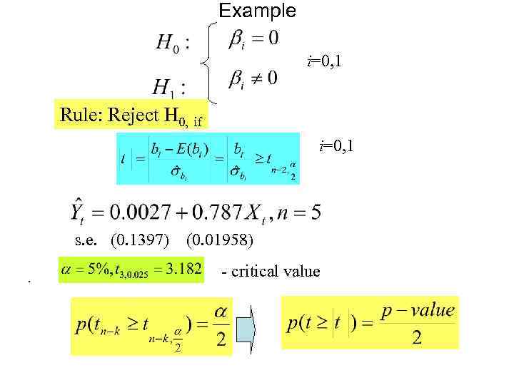Example i=0, 1 Rule: Reject H 0, if i=0, 1 s. e. (0. 1397). (0. 01958) - critical value

Example s. e. (0. 1397) . (0. 01958)

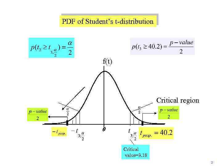PDF of Student’s t-distribution f(t) Critical region 0 t Critical value=3. 18 2

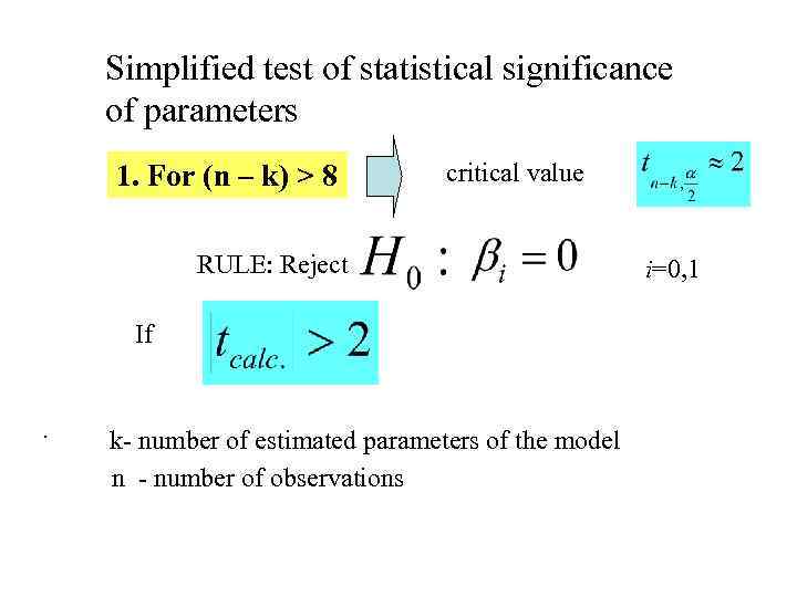Simplified test of statistical significance of parameters 1. For (n – k) > 8 critical value RULE: Reject If . k- number of estimated parameters of the model n - number of observations i=0, 1

Test for parameters’ statistical significance 2. When n > 30 RULE: We reject : at α = 10% , if at α = 5% , if. at α = 1% , if i=0, 1

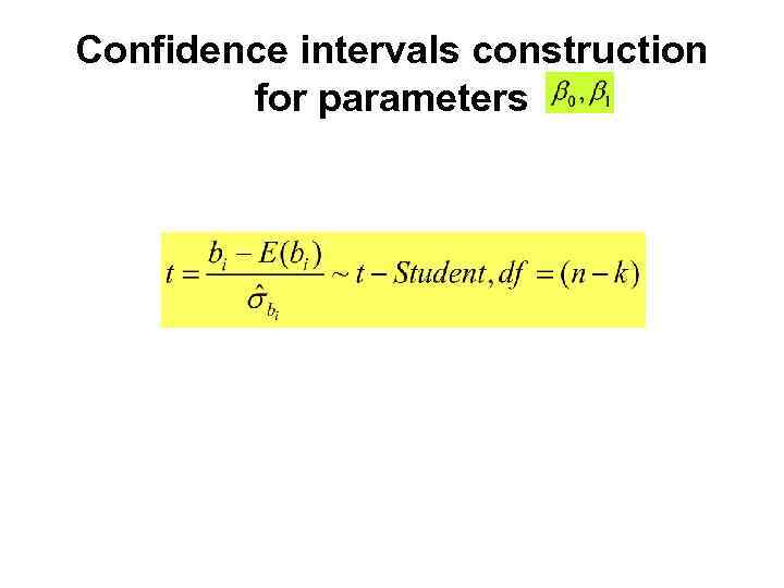Confidence intervals construction for parameters

A 95% confidence interval of such that is an interval centered around with probability 95% PDF of Student’s t-distribution f(t) (1 -α) 0 Critical region t 2

.

.

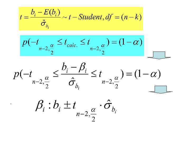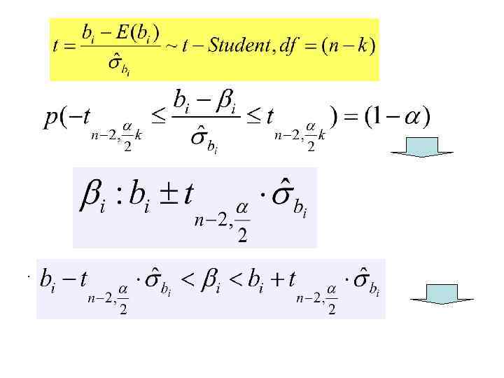Exercise • Construct confidence intervals for parameter

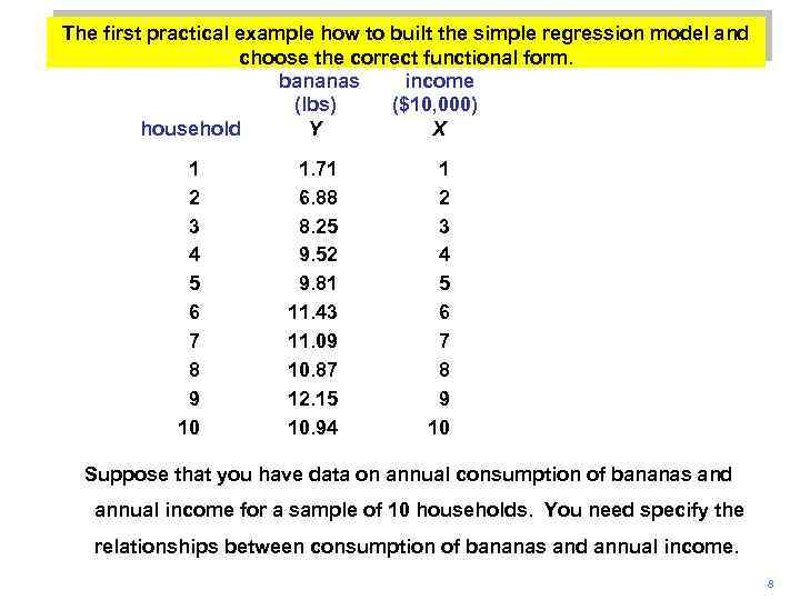The first practical example how to built the simple regression model and choose the correct functional form. bananas income (lbs) ($10, 000) household Y X 1 2 3 4 5 6 7 8 9 10 1. 71 6. 88 8. 25 9. 52 9. 81 11. 43 11. 09 10. 87 12. 15 10. 94 1 2 3 4 5 6 7 8 9 10 Suppose that you have data on annual consumption of bananas and annual income for a sample of 10 households. You need specify the relationships between consumption of bananas and annual income. 8

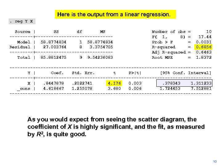Here is the output from a linear regression. . reg Y X Source | SS df MS -----+---------------Model | 58. 8774834 1 58. 8774834 Residual | 27. 003764 8 3. 3754705 -----+---------------Total | 85. 8812475 9 9. 54236083 Number of obs F( 1, 8) Prob > F R-squared Adj R-squared Root MSE = = = 10 17. 44 0. 0031 0. 6856 0. 6463 1. 8372 ---------------------------------------Y | Coef. Std. Err. t P>|t| [95% Conf. Interval] -----+----------------------------------X |. 8447878. 2022741 4. 176 0. 003. 378343 1. 311233 _cons | 4. 618667 1. 255078 3. 680 0. 006 1. 724453 7. 512881 --------------------------------------- As you would expect from seeing the scatter diagram, the coefficient of X is highly significant, and the fit, as measured by R 2, is quite good. 10