Lecture 3 Introductory Econometrics INTRODUCTION TO LINEAR REGRESSION

Lecture 3 Introductory Econometrics INTRODUCTION TO LINEAR REGRESSION MODEL II September 20, 2014

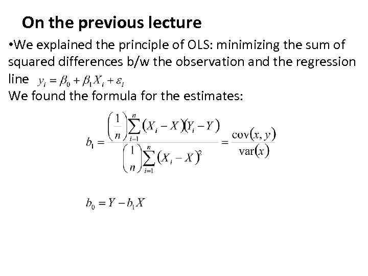On the previous lecture • We explained the principle of OLS: minimizing the sum of squared differences b/w the observation and the regression line We found the formula for the estimates:

On the previous lecture • We explained that the stochastic error term must be present in a regression equation because of: – – 1. omission of many minor influences (unavailable data) 2. measurement error 3. possibly incorrect functional form 4. stochastic character of unpredictable human behavior • Remember that all of these factors are included in the error term and may alter its properties • The properties of the error term determine the properties of the estimates

On today’s lecture • We will study PRM (Population Regression Model vs SRM (Sample Regression Model) • We will list the assumptions about the error term (ei) and the explanatory variables (Xi) that are required in classical regression models • We will derive the properties of the OLS estimate (b 0, b 1) for the case when classical assumptions hold • We will show that under these assumption, OLS is the best estimator available for regression models • The rest of the course will mostly deal in one way or another with the question what to do when one of the classical assumptions is not met

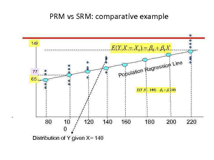
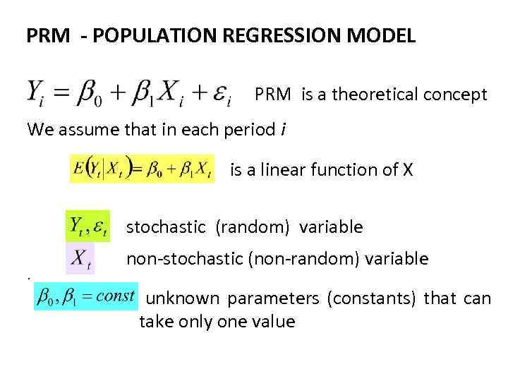PRM - POPULATION REGRESSION MODEL PRM is a theoretical concept We assume that in each period i is a linear function of X stochastic (random) variable. non-stochastic (non-random) variable unknown parameters (constants) that can take only one value

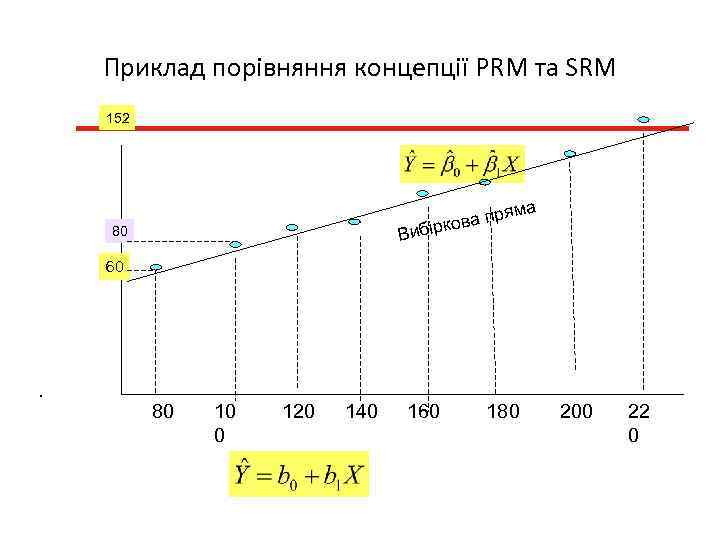
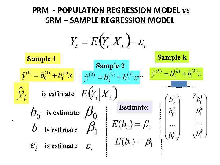PRM - POPULATION REGRESSION MODEL vs SRM – SAMPLE REGRESSION MODEL Sample 1 Sample k Sample 2. . . is estimate Estimate:

PRM - POPULATION REGRESSION MODEL const Stoch. variable const Random variable, which measures uncertainty Statistical relation Assumptions: 1. Х influences on Y, but Y doesn’t influence on Х 2. Х is non-stochastic variable, Х doesn’t change from sample. to sample (Xs are fixed in repeated sampling) Goal: estimate - linear population regression model on the basis of sample Хi та Yi

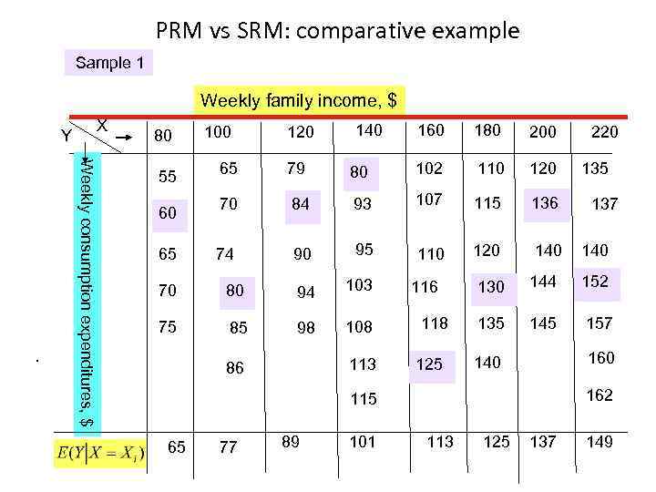
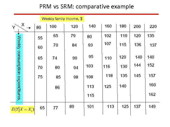PRM vs SRM: comparative example Weekly family income, $ X Y 80 Weekly consumption expenditures, 55 60 65 100 65 120 79 140 160 180 200 80 102 110 120 70 84 93 107 115 136 74 90 95 110 120 140 70 80 94 103 75 85 98 108 113 86 118 125 130 144 135 145 77 89 101 135 137 140 152 157 160 140 162 115 65 220 113 125 137 149

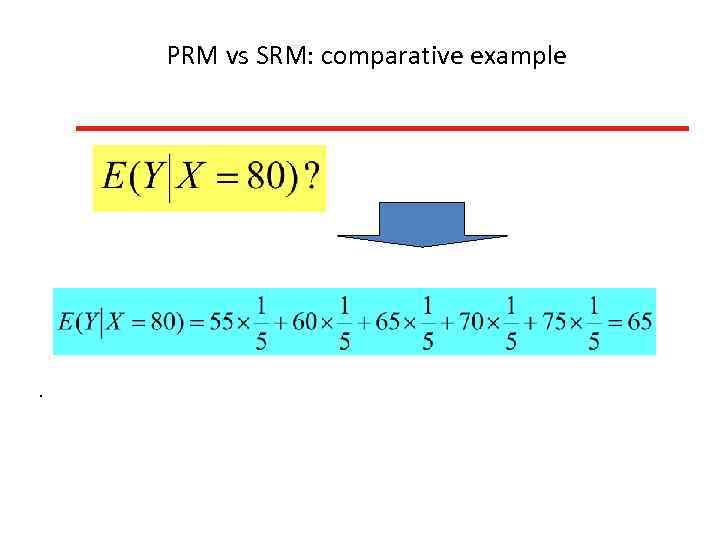
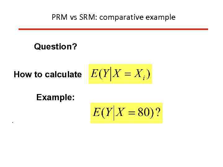PRM vs SRM: comparative example Question? How to calculate Example: .

PRM vs SRM: comparative example .

PRM vs SRM: comparative example 149 ine sion L gres on Re pulati 77 Po 65 . 80 10 0 120 140 Distribution of Y given X= 140 160 180 200 220

PRM vs SRM: comparative example Sample 1 Weekly family income, $ X Y Weeklу consumption expenditures, $ . 80 55 60 65 100 65 120 79 140 160 180 200 80 102 110 120 70 84 93 107 115 136 74 90 95 110 120 140 70 80 94 103 75 85 98 108 113 86 118 125 130 144 135 145 77 89 101 135 137 140 152 157 160 140 162 115 65 220 113 125 137 149

Приклад порівняння концепції PRM та SRM 152 яма пр іркова Виб 80 60 . 80 10 0 120 140 160 180 200 22 0

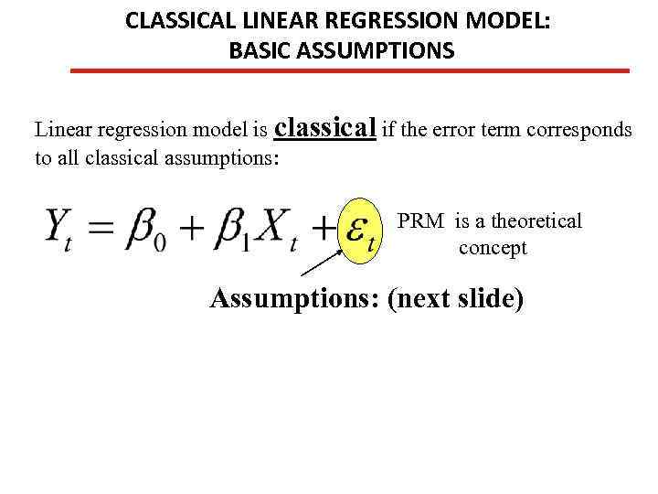CLASSICAL LINEAR REGRESSION MODEL: BASIC ASSUMPTIONS Linear regression model is classical if the error term corresponds to all classical assumptions: PRM is a theoretical concept Assumptions: (next slide)

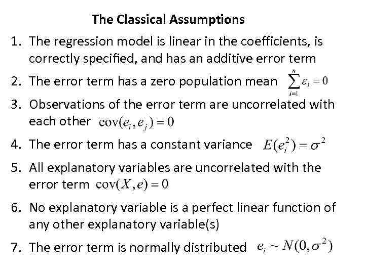The Classical Assumptions 1. The regression model is linear in the coefficients, is correctly specified, and has an additive error term 2. The error term has a zero population mean 3. Observations of the error term are uncorrelated with each other 4. The error term has a constant variance 5. All explanatory variables are uncorrelated with the error term 6. No explanatory variable is a perfect linear function of any other explanatory variable(s) 7. The error term is normally distributed

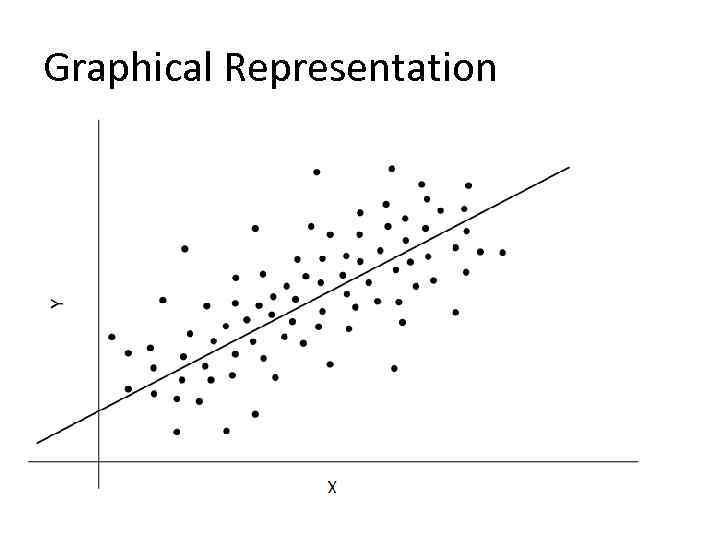Graphical Representation

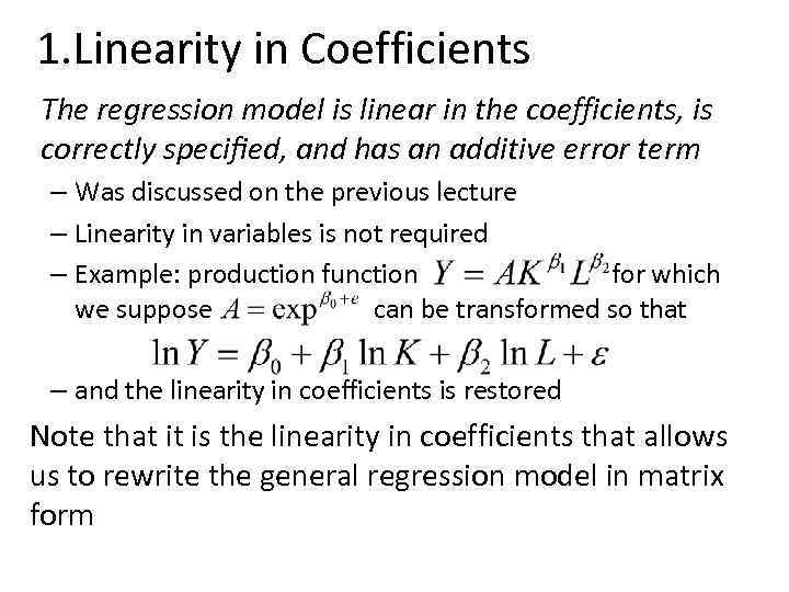1. Linearity in Coefficients The regression model is linear in the coefficients, is correctly specified, and has an additive error term – Was discussed on the previous lecture – Linearity in variables is not required – Example: production function for which we suppose can be transformed so that – and the linearity in coefficients is restored Note that it is the linearity in coefficients that allows us to rewrite the general regression model in matrix form

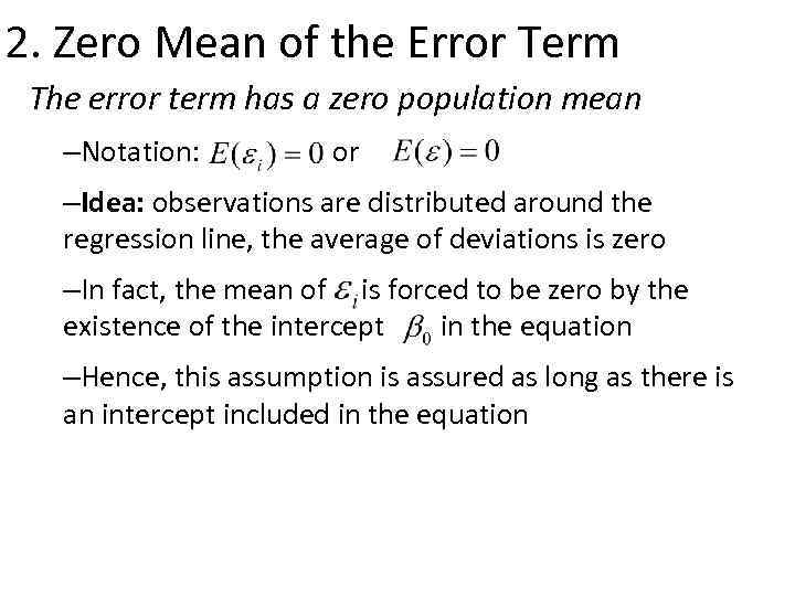2. Zero Mean of the Error Term The error term has a zero population mean –Notation: or –Idea: observations are distributed around the regression line, the average of deviations is zero –In fact, the mean of is forced to be zero by the existence of the intercept in the equation –Hence, this assumption is assured as long as there is an intercept included in the equation

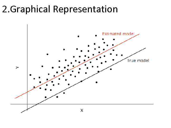2. Graphical Representation

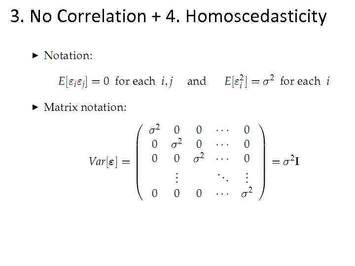
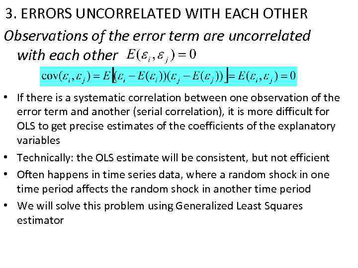3. ERRORS UNCORRELATED WITH EACH OTHER Observations of the error term are uncorrelated with each other • If there is a systematic correlation between one observation of the error term and another (serial correlation), it is more difficult for OLS to get precise estimates of the coefficients of the explanatory variables • Technically: the OLS estimate will be consistent, but not efficient • Often happens in time series data, where a random shock in one time period affects the random shock in another time period • We will solve this problem using Generalized Least Squares estimator

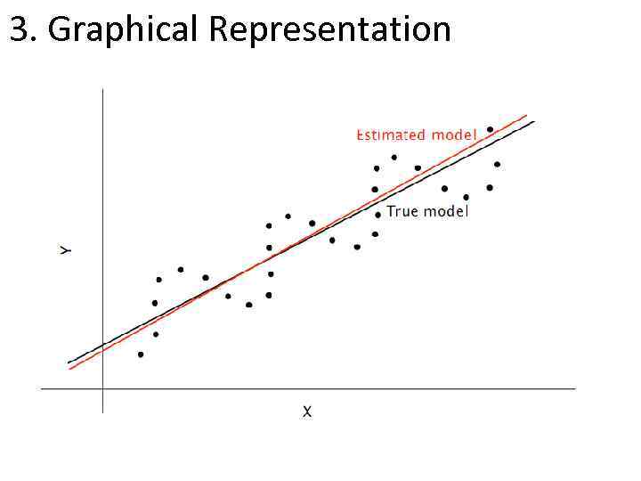3. Graphical Representation

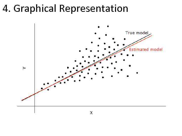
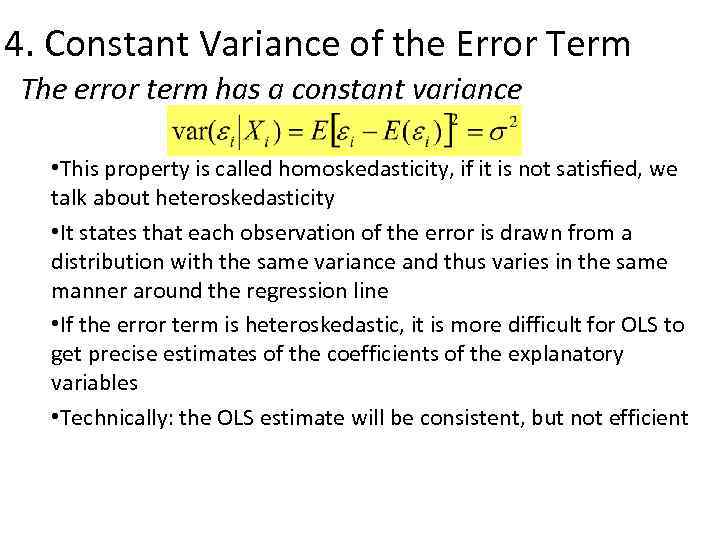4. Constant Variance of the Error Term The error term has a constant variance • This property is called homoskedasticity, if it is not satisfied, we talk about heteroskedasticity • It states that each observation of the error is drawn from a distribution with the same variance and thus varies in the same manner around the regression line • If the error term is heteroskedastic, it is more difficult for OLS to get precise estimates of the coefficients of the explanatory variables • Technically: the OLS estimate will be consistent, but not efficient

4. Constant Variance of the Error Term • Heteroskedasticity is often present in cross-sectional data • Example: Analysis of household consumption patterns • Variance of the consumption of certain goods might be greater for higher-income households • These have more discretionary income than do lowerincome households • We will solve this problem using Hull-White robust standard errors

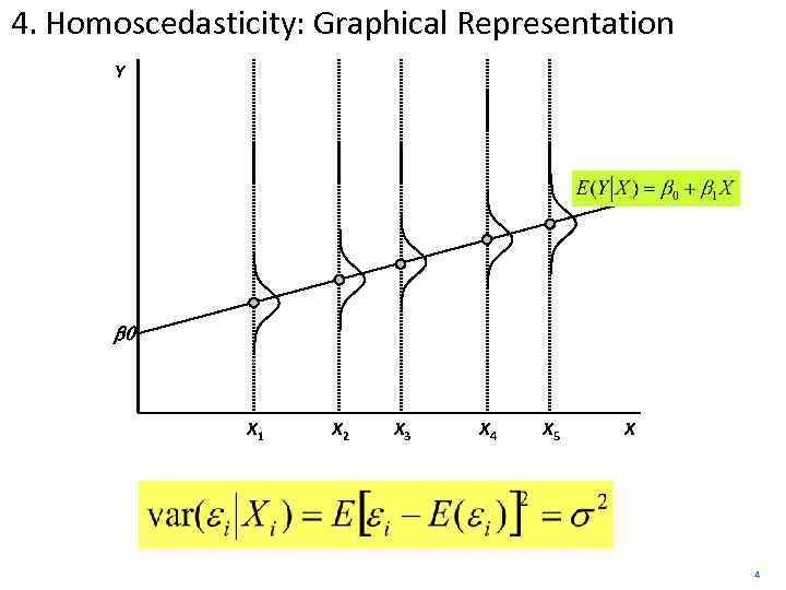4. Homoscedasticity: Graphical Representation Y b 0 X 1 X 2 X 3 X 4 X 5 X 4

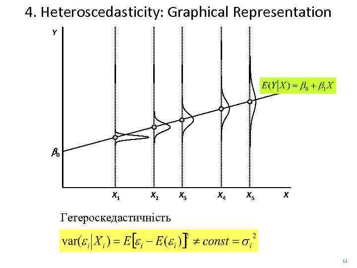4. Heteroscedasticity: Graphical Representation Y b 0 X 1 X 2 X 3 X 4 X 5 X Гетероскедастичність 11

4. Graphical Representation

3. No Correlation + 4. Homoscedasticity

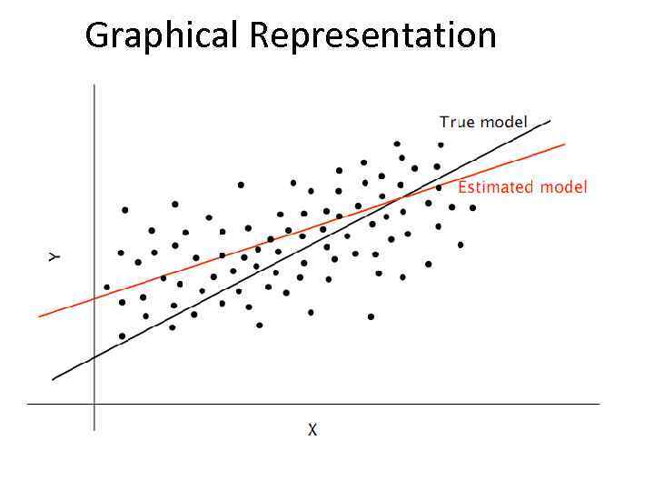
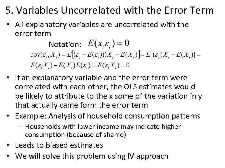5. Variables Uncorrelated with the Error Term • All explanatory variables are uncorrelated with the error term Notation: • If an explanatory variable and the error term were correlated with each other, the OLS estimates would be likely to attribute to the x some of the variation in y that actually came form the error term • Example: Analysis of household consumption patterns – Households with lower income may indicate higher consumption (because of shame) • Leads to biased estimates • We will solve this problem using IV approach

Graphical Representation

6. Linearly Independent Variables No explanatory variable is a perfect linear function of any other explanatory variable(s) – If this condition does not hold, we talk about (multi)collinearity – In this case, the OLS model is incapable to distinguish one variable from the other – Technical consequence: does not exist – Example: we include both real and nominal interest rate in a model with constant inflation – Solution: drop one of the variables

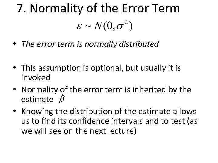7. Normality of the Error Term • The error term is normally distributed • This assumption is optional, but usually it is invoked • Normality of the error term is inherited by the estimate • Knowing the distribution of the estimate allows us to find its confidence intervals and to test (as we will see on the next lecture)

Gauss-Markov Theorem Given Classical Assumptions, the OLS estimator of would be BLUE For example - Best Linear Unbiased Estimator is BLUЕ estimate of 1. Linearity For example, . or could be expressed as a linear function of Y

Gauss-Markov Theorem (2) BLUE - Best linear unbiased estimator 2. Consistency When no explanatory variables are correlated with the error term , OLS estimate is consistent: In other words: as the number of observations increases, the estimate converges to the true value. of the coefficient Consistency is the most (!!!) important property of an estimate !!!!!!!!!!

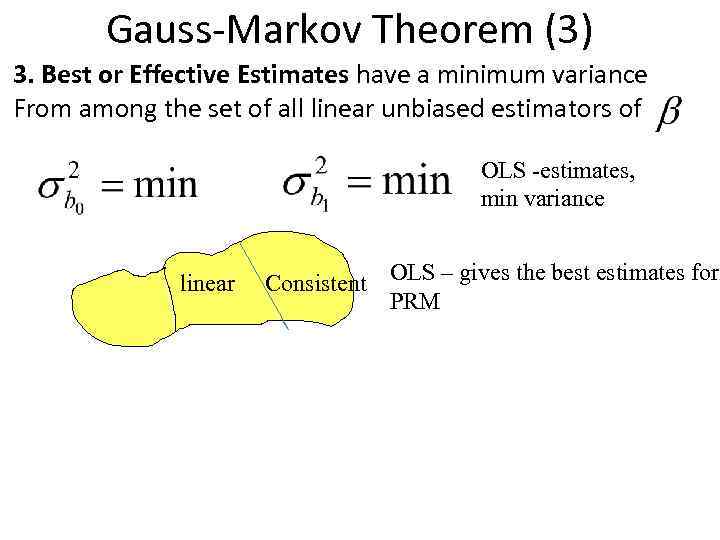Gauss-Markov Theorem (3) 3. Best or Effective Estimates have a minimum variance From among the set of all linear unbiased estimators of OLS -estimates, min variance linear Consistent OLS – gives the best estimates for PRM

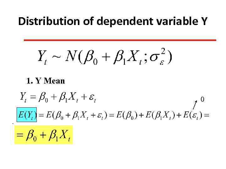Distribution of dependent variable Y 1. Y Mean 0.

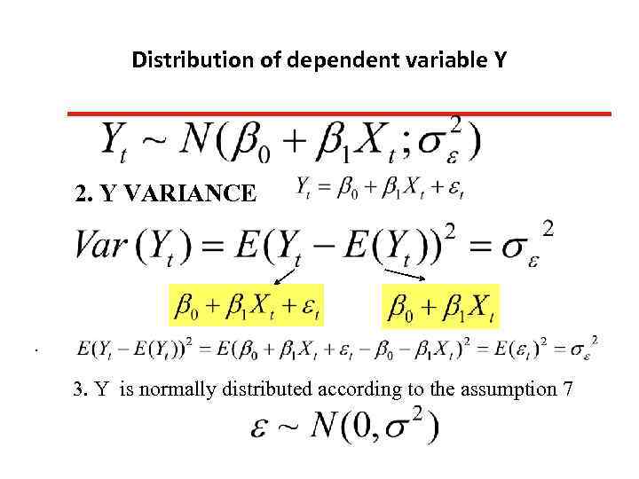Distribution of dependent variable Y 2. Y VARIANCE . 3. Y is normally distributed according to the assumption 7

Summary • We have listed the classical assumptions of regression models: – model linear in parameters, explanatory variables linearly – independent – (normally distributed) error term with zero mean and constant variance, no serial autocorrelation – no correlation between error term and explanatory variables • We have shown that if these assumptions hold, OLS estimate is – – Consistent Unbiased Efficient Normally distributed

To be Continued…. . )) • Next lecture: • OLS formula, formula for variance and expected value of parameters • hypothesis testing • correlation and determination coefficients • Home assignment #1: • Deadline: Tuesday, October 1, 11 a. m. 6 -406 • Individual, submit hard copy => no e-mails.