87171dbe05fbc2ecdc2100fe9070fe7d.ppt
- Количество слайдов: 21
 Lecture 2, Thursday, Aug. 24. Population ecology is a major subfield of ecology—one that deals with the dynamics of species populations and how these populations interact with the environment. http: //en. wikipedia. org/wiki/Populatio n_ecology
 Uncontrolled E. Coli growth A single cell of the bacterium Escherichia coli, would, under ideal circumstances, divide every twenty min utes. … it can be shown that in a single day, one cell of E. coli could produce a super colony equal in size and weight to the entire planet earth. E. coli cells are elongated, 1 -2 µm in length and 0. 1 -0. 5 µm in diameter. (Exercise 1. 2)-------M. Crichton (1969), The Andromeda Strain (Dell, New York, p. 247).
 Reading homework • Required Reading: section 4. 1, page 116 121. • Suggested Reading: Thomas Malthus: An Essay on the Principles of Population Growth, 1798. http: //www. marxists. org/reference/subject/econo mics/malthus/ • Suggested Reading: Georgyi Frantsevitch Gause: The Struggle for Existence, 1934. Free obline http: //www. ggause. com/Contgau. htm. Buy for $35 at Amazon. com. http: //www. amazon. com/gp/product/0486495205 /102 -6000505 -7050558? v=glance&n=283155
 Four major processes • The four major processes that regulate population growths are: birth (B, +), death (D, -), immigration (I, +) and emigration (E, -) (where B is the number of births, D is the number of deaths, I is the number of immigrants and E is number of emigrants). We assume first that the population grows in a closed environment. Hence we will ignore both the immigration and emigration processes.
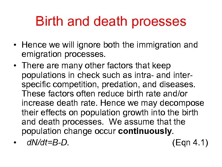 Birth and death proesses • Hence we will ignore both the immigration and emigration processes. • There are many other factors that keep populations in check such as intra- and interspecific competition, predation, and diseases. These factors often reduce birth rate and/or increase death rate. Hence we may decompose their effects on population growth into the birth and death processes. We assume that the population change occur continuously. • d. N/dt=B D. (Eqn 4. 1)
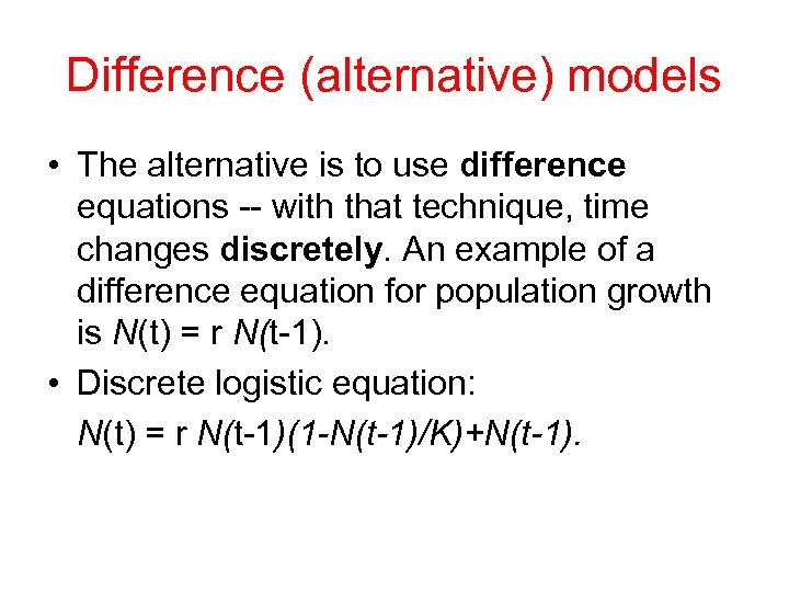 Difference (alternative) models • The alternative is to use difference equations -- with that technique, time changes discretely. An example of a difference equation for population growth is N(t) = r N(t-1). • Discrete logistic equation: N(t) = r N(t-1)(1 N(t 1)/K)+N(t 1).
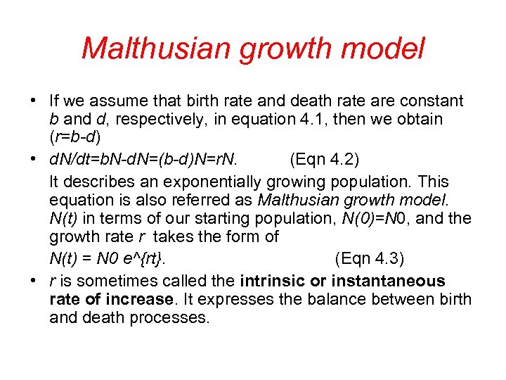 Malthusian growth model • If we assume that birth rate and death rate are constant b and d, respectively, in equation 4. 1, then we obtain (r=b d) • d. N/dt=b. N d. N=(b d)N=r. N. (Eqn 4. 2) It describes an exponentially growing population. This equation is also referred as Malthusian growth model. N(t) in terms of our starting population, N(0)=N 0, and the growth rate r takes the form of N(t) = N 0 e^{rt}. (Eqn 4. 3) • r is sometimes called the intrinsic or instantaneous rate of increase. It expresses the balance between birth and death processes.
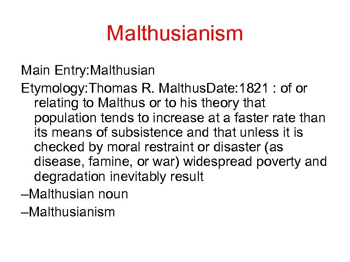 Malthusianism Main Entry: Malthusian Etymology: Thomas R. Malthus. Date: 1821 : of or relating to Malthus or to his theory that population tends to increase at a faster rate than its means of subsistence and that unless it is checked by moral restraint or disaster (as disease, famine, or war) widespread poverty and degradation inevitably result –Malthusian noun –Malthusianism
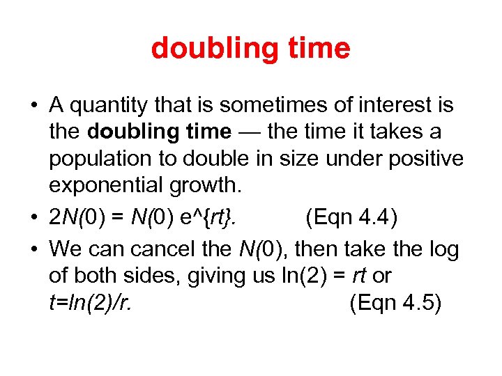 doubling time • A quantity that is sometimes of interest is the doubling time — the time it takes a population to double in size under positive exponential growth. • 2 N(0) = N(0) e^{rt}. (Eqn 4. 4) • We cancel the N(0), then take the log of both sides, giving us ln(2) = rt or t=ln(2)/r. (Eqn 4. 5)
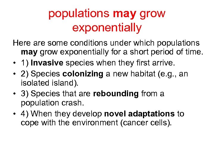 populations may grow exponentially Here are some conditions under which populations may grow exponentially for a short period of time. • 1) Invasive species when they first arrive. • 2) Species colonizing a new habitat (e. g. , an isolated island). • 3) Species that are rebounding from a population crash. • 4) When they develop novel adaptations to cope with the environment (cancer cells).
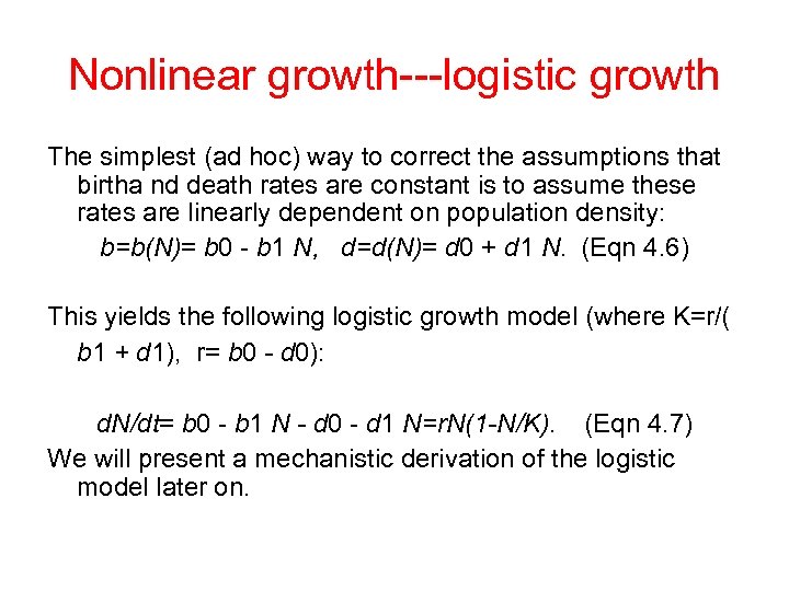 Nonlinear growth---logistic growth The simplest (ad hoc) way to correct the assumptions that birtha nd death rates are constant is to assume these rates are linearly dependent on population density: b=b(N)= b 0 - b 1 N, d=d(N)= d 0 + d 1 N. (Eqn 4. 6) This yields the following logistic growth model (where K=r/( b 1 + d 1), r= b 0 d 0): d. N/dt= b 0 - b 1 N d 0 - d 1 N=r. N(1 N/K). (Eqn 4. 7) We will present a mechanistic derivation of the logistic model later on.
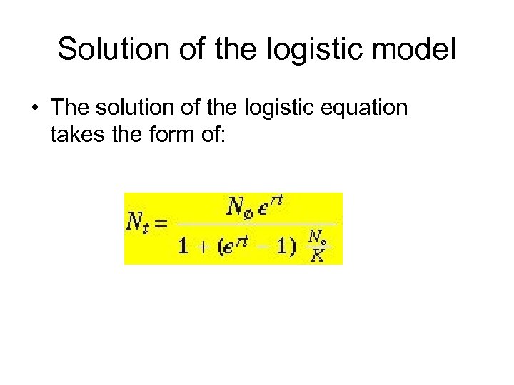 Solution of the logistic model • The solution of the logistic equation takes the form of:
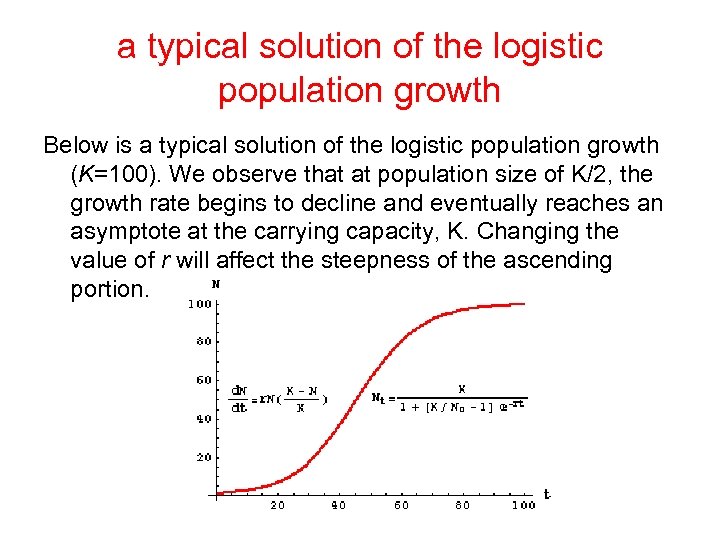 a typical solution of the logistic population growth Below is a typical solution of the logistic population growth (K=100). We observe that at population size of K/2, the growth rate begins to decline and eventually reaches an asymptote at the carrying capacity, K. Changing the value of r will affect the steepness of the ascending portion.
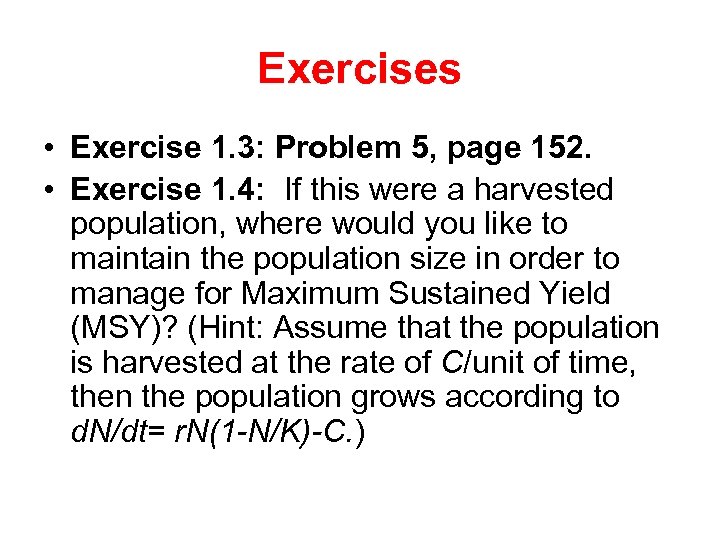 Exercises • Exercise 1. 3: Problem 5, page 152. • Exercise 1. 4: If this were a harvested population, where would you like to maintain the population size in order to manage for Maximum Sustained Yield (MSY)? (Hint: Assume that the population is harvested at the rate of C/unit of time, then the population grows according to d. N/dt= r. N(1 N/K) C. )
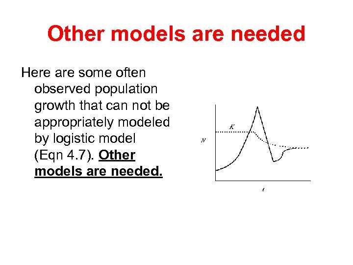 Other models are needed Here are some often observed population growth that can not be appropriately modeled by logistic model (Eqn 4. 7). Other models are needed.
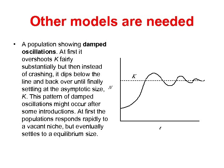 Other models are needed • A population showing damped oscillations. At first it overshoots K fairly substantially but then instead of crashing, it dips below the line and back over until finally settling at the asymptotic size, K. This pattern of damped oscillations might occur after some introductions. At first the populations responds rapidly to a vacant niche, but eventually settles to a equilibrium size.
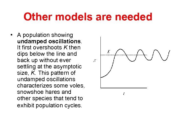 Other models are needed • A population showing undamped oscillations. It first overshoots K then dips below the line and back up without ever settling at the asymptotic size, K. This pattern of undamped oscillations characterizes some voles, snowshoe hares and other species that tend to exhibit population cycles.
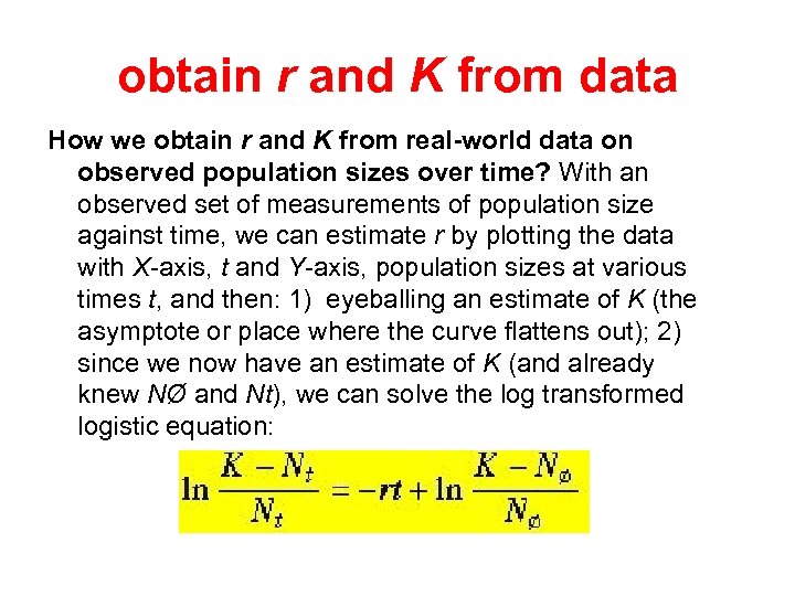 obtain r and K from data How we obtain r and K from real-world data on observed population sizes over time? With an observed set of measurements of population size against time, we can estimate r by plotting the data with X-axis, t and Y-axis, population sizes at various times t, and then: 1) eyeballing an estimate of K (the asymptote or place where the curve flattens out); 2) since we now have an estimate of K (and already knew NØ and Nt), we can solve the log transformed logistic equation:
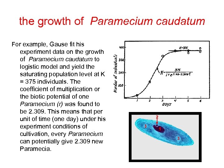 the growth of Paramecium caudatum For example, Gause fit his experiment data on the growth of Paramecium caudatum to logistic model and yield the saturating population level at K = 375 individuals. The coefficient of multiplication or the biotic potential of one Paramecium (r) was found to be 2. 309. This means that per unit of time (one day) under his experiment conditions of cultivation, every Paramecium can potentially give 2. 309 new Paramecia.


