Lecture 2 Introductory Econometrics INTRODUCTION TO LINEAR REGRESSSION

Lecture 2 Introductory Econometrics INTRODUCTION TO LINEAR REGRESSSION MODEL 1 September, 13 2014

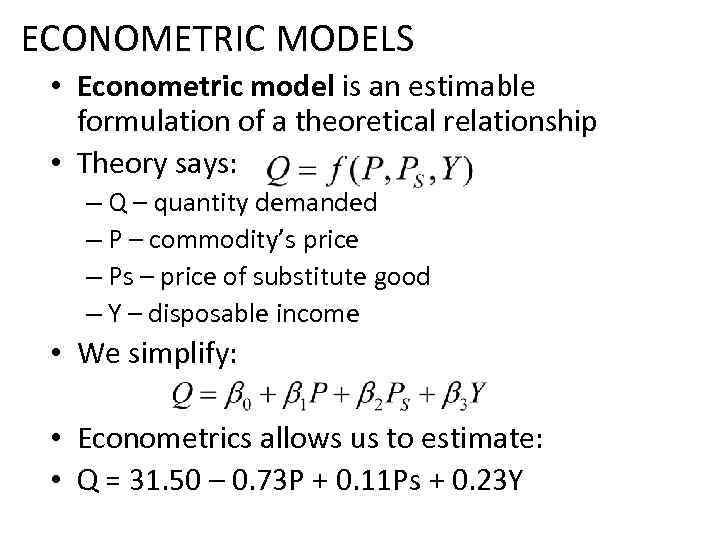ECONOMETRIC MODELS • Econometric model is an estimable formulation of a theoretical relationship • Theory says: – Q – quantity demanded – P – commodity’s price – Ps – price of substitute good – Y – disposable income • We simplify: • Econometrics allows us to estimate: • Q = 31. 50 – 0. 73 P + 0. 11 Ps + 0. 23 Y

ECONOMETRIC MODELS • Today’s econometrics deals with different, even very general models • During the course we will cover just linear regression models • We will see how these models are estimated by: üOLS (Ordinary Least Squares) üGLS (Generalized Least Squares) üInstrumental variables • We’ll perform estimations on different types of data

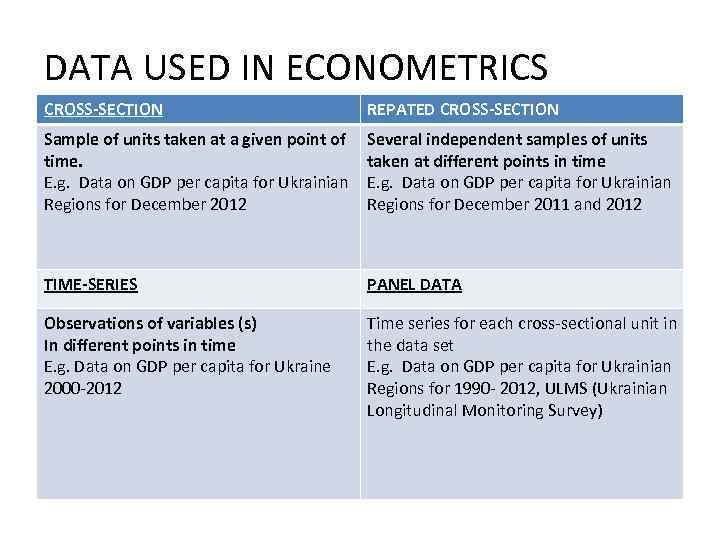DATA USED IN ECONOMETRICS CROSS-SECTION REPATED CROSS-SECTION Sample of units taken at a given point of time. E. g. Data on GDP per capita for Ukrainian Regions for December 2012 Several independent samples of units taken at different points in time E. g. Data on GDP per capita for Ukrainian Regions for December 2011 and 2012 TIME-SERIES PANEL DATA Observations of variables (s) In different points in time E. g. Data on GDP per capita for Ukraine 2000 -2012 Time series for each cross-sectional unit in the data set E. g. Data on GDP per capita for Ukrainian Regions for 1990 - 2012, ULMS (Ukrainian Longitudinal Monitoring Survey)

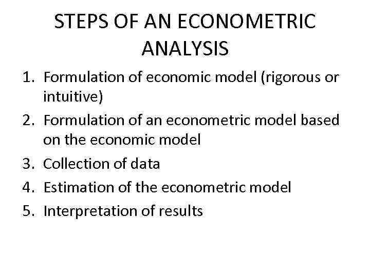STEPS OF AN ECONOMETRIC ANALYSIS 1. Formulation of economic model (rigorous or intuitive) 2. Formulation of an econometric model based on the economic model 3. Collection of data 4. Estimation of the econometric model 5. Interpretation of results

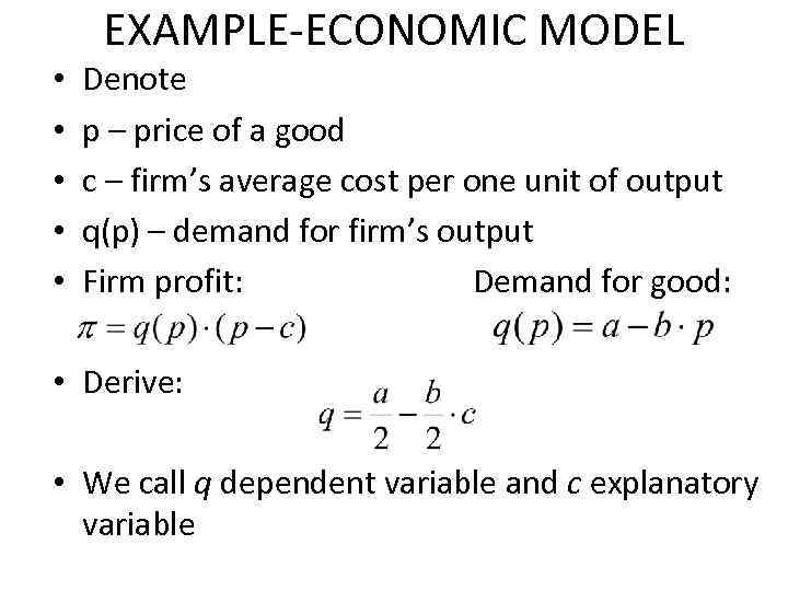EXAMPLE-ECONOMIC MODEL • • • Denote p – price of a good c – firm’s average cost per one unit of output q(p) – demand for firm’s output Firm profit: Demand for good: • Derive: • We call q dependent variable and c explanatory variable

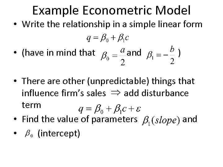Example Econometric Model • Write the relationship in a simple linear form • (have in mind that and ) • There are other (unpredictable) things that influence firm’s sales add disturbance term • Find the value of parameters and • (intercept)

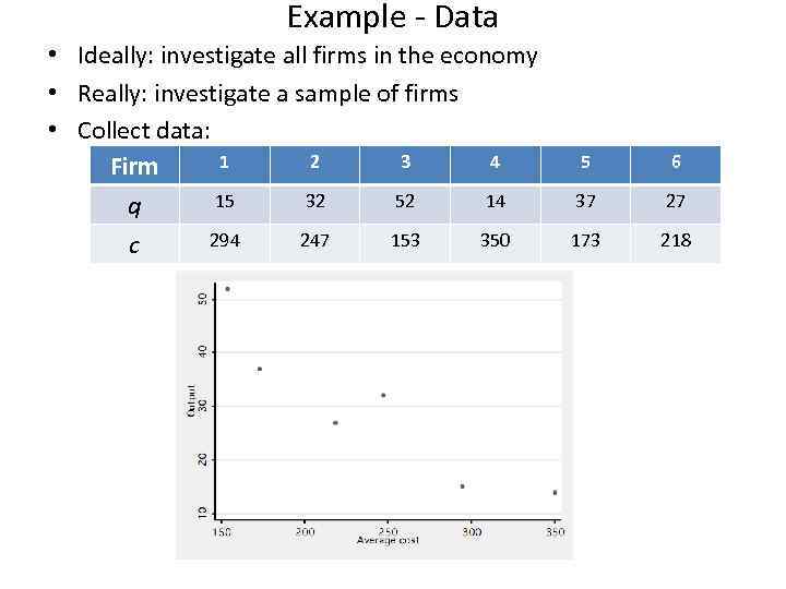Example - Data • Ideally: investigate all firms in the economy • Really: investigate a sample of firms • Collect data: 1 2 3 4 Firm 15 32 52 14 q 294 247 153 350 c 5 6 37 27 173 218

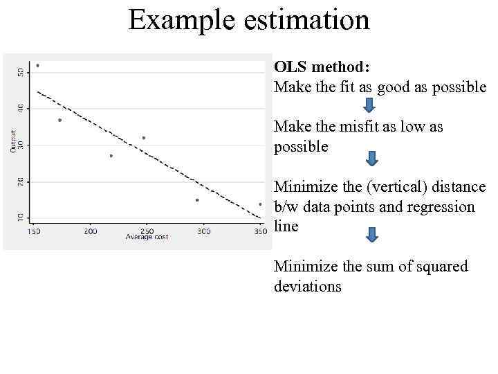Example estimation OLS method: Make the fit as good as possible Make the misfit as low as possible Minimize the (vertical) distance b/w data points and regression line Minimize the sum of squared deviations

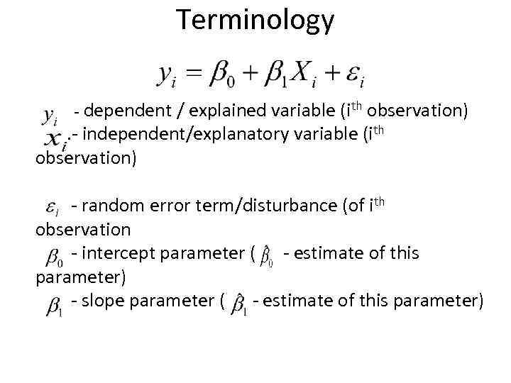Terminology - dependent / explained variable (ith observation) . - independent/explanatory variable (ith observation) - random error term/disturbance (of ith observation - intercept parameter ( - estimate of this parameter) - slope parameter ( - estimate of this parameter)

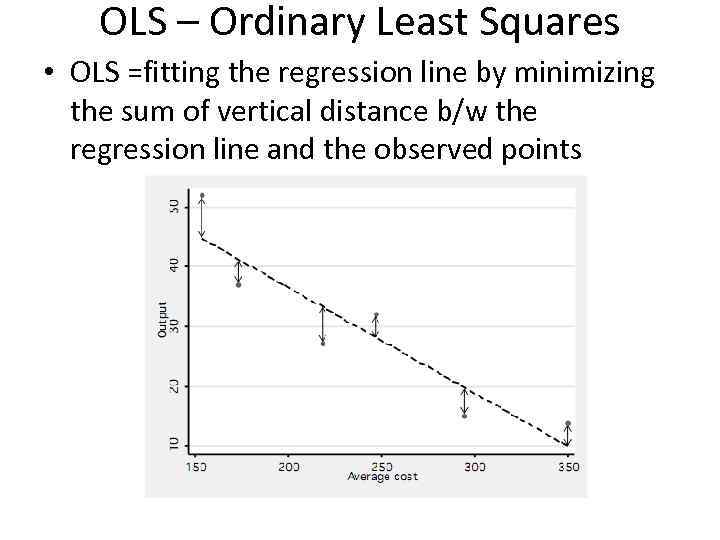OLS – Ordinary Least Squares • OLS =fitting the regression line by minimizing the sum of vertical distance b/w the regression line and the observed points

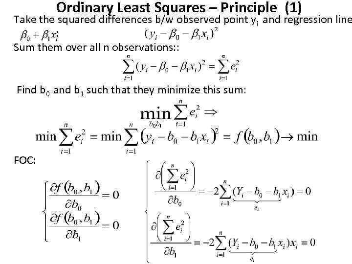Ordinary Least Squares – Principle (1) Take the squared differences b/w observed point yi and regression line : Sum them over all n observations: : Find b 0 and b 1 such that they minimize this sum: FOC:

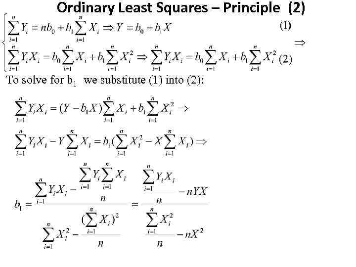Ordinary Least Squares – Principle (2) To solve for b 1 we substitute (1) into (2):

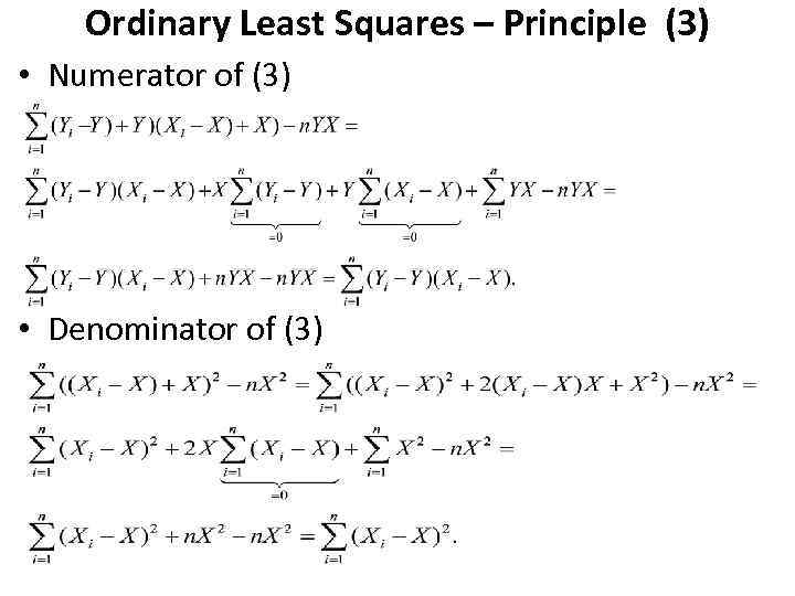Ordinary Least Squares – Principle (3) • Numerator of (3) • Denominator of (3)

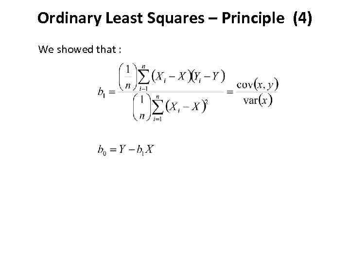Ordinary Least Squares – Principle (4) We showed that :

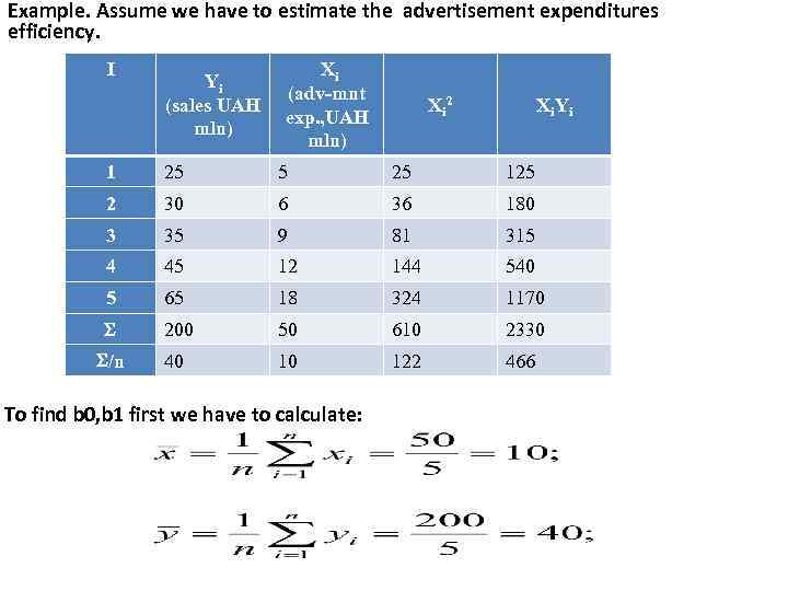Example. Assume we have to estimate the advertisement expenditures efficiency. I Yi (sales UAH mln) Xi (adv-mnt exp. , UAH mln) Xi 2 Xi. Yi 1 25 5 25 125 2 30 6 36 180 3 35 9 81 315 4 45 12 144 540 5 65 18 324 1170 200 50 610 2330 /n 40 10 122 466 To find b 0, b 1 first we have to calculate:

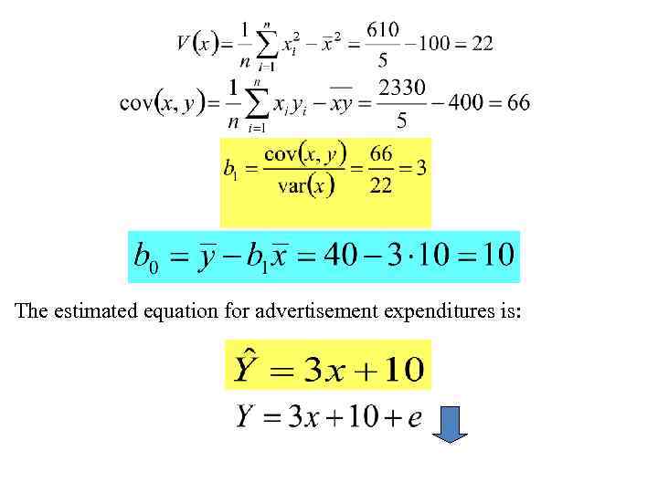The estimated equation for advertisement expenditures is:

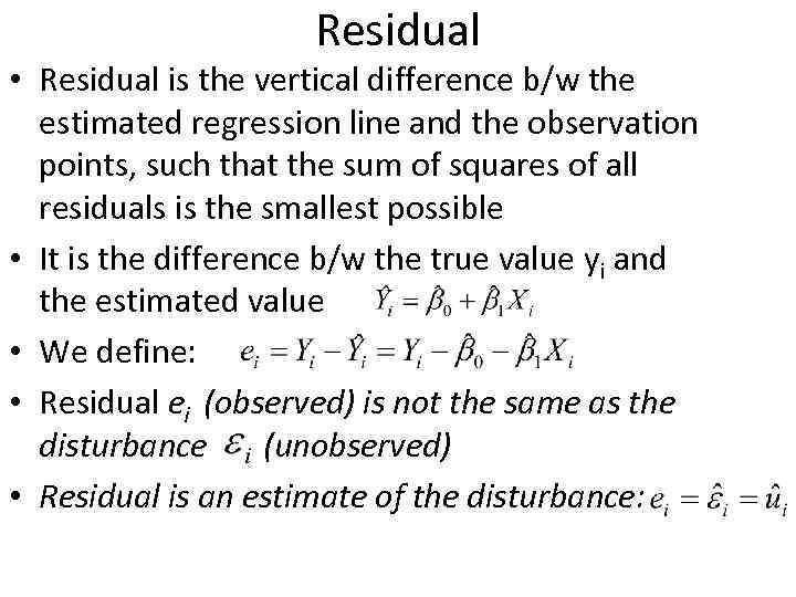Residual • Residual is the vertical difference b/w the estimated regression line and the observation points, such that the sum of squares of all residuals is the smallest possible • It is the difference b/w the true value yi and the estimated value • We define: • Residual ei (observed) is not the same as the disturbance (unobserved) • Residual is an estimate of the disturbance:

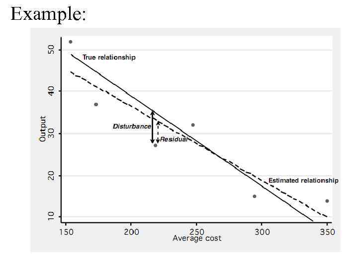Example:

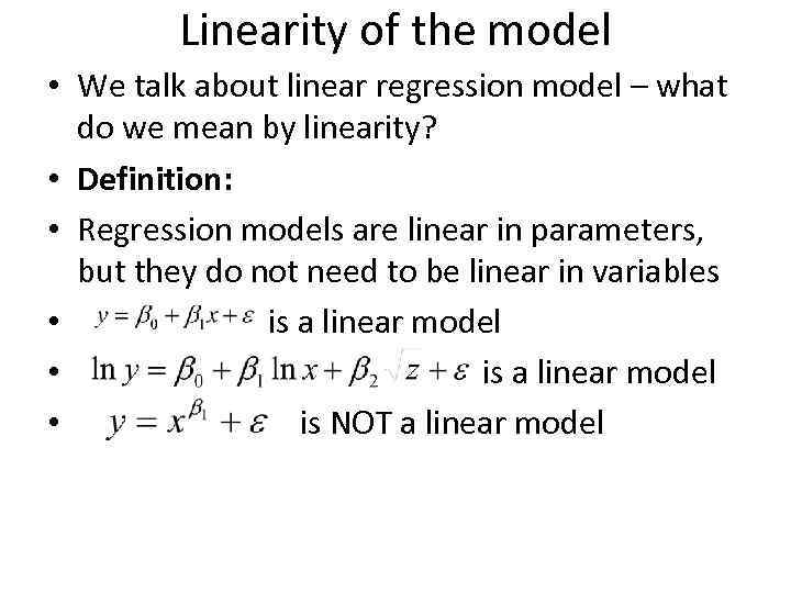Linearity of the model • We talk about linear regression model – what do we mean by linearity? • Definition: • Regression models are linear in parameters, but they do not need to be linear in variables • is a linear model • is NOT a linear model

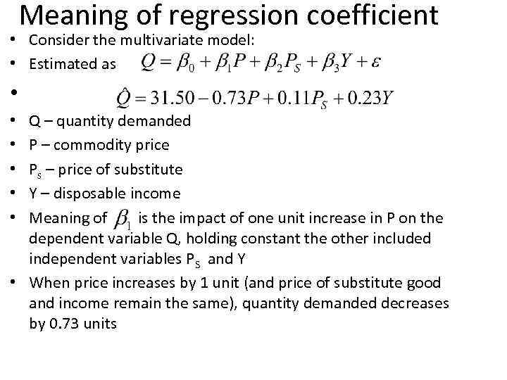Meaning of regression coefficient • Consider the multivariate model: • Estimated as • Q – quantity demanded P – commodity price Ps – price of substitute Y – disposable income Meaning of is the impact of one unit increase in P on the dependent variable Q, holding constant the other included independent variables PS and Y • When price increases by 1 unit (and price of substitute good and income remain the same), quantity demanded decreases by 0. 73 units • • •

Behind the error term • The stochastic error term must be present in a regression equation because of: 1. 2. 3. 4. Omission of many minor influences (unavailable data) Measurement error Possibly incorrect functional form Stochastic character of unpredictable human behavior • Remember that all of these factors are included in the error term and may alter the properties • The properties of the error term determine the properties of the estimates

Summary • We have learned that an econometric analysis consists of 1. Definition of the model 2. Estimation 3. Interpretation • We have explained the principle of OLS: minimizing the sum of squared differences b/w the observation and the regression line

To be continued …… • On the next lecture, we will specify the properties of OLS estimator • On the coming practice session, we will • Continue with Stata • Show some examples of regression models