Lecture 2 Descriptive Statistics GOW 1

Lecture 2 Descriptive Statistics GOW 1

• Measures of location GOW

• Numerical measures of location, dispersion, shape, and association are introduced. • If the measures are computed for data from a sample, they are called sample statistics. • If the measures are computed for data from a population, they are called population parameters. GOW

Measures of Central Tendency and Measures of Dispersion (Variation) • Measures of Central Tendency describes the center point of our data set with a single value. Examples are: mean, median, mode • Measures of Dispersion show much scatter or variation exists in the data Examples to be discussed. GOW 4

MEAN • GOW

Mean or Average The mean or average is the most common measure of central tendency and is calculated by adding all values in our data set and then dividing this result by the number of observations GOW 6

Mean or Average The mean or average is the most common measure of central tendency and is calculated by adding all values in our data set and then dividing this result by the number of observations GOW 7

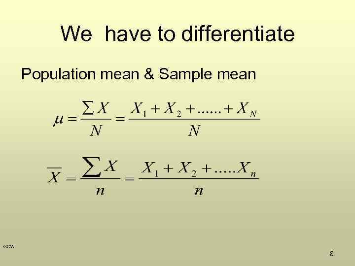We have to differentiate Population mean & Sample mean GOW 8

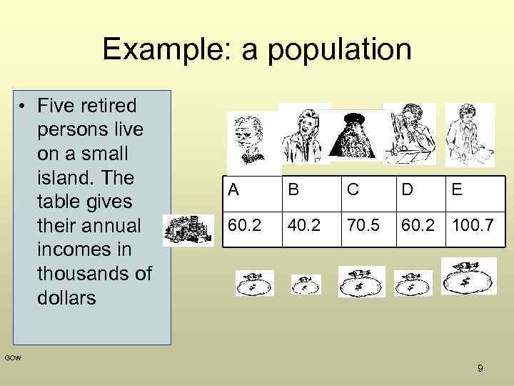Example: a population • Five retired persons live on a small island. The table gives their annual incomes in thousands of dollars A B C D E 60. 2 40. 2 70. 5 60. 2 100. 7 GOW 9

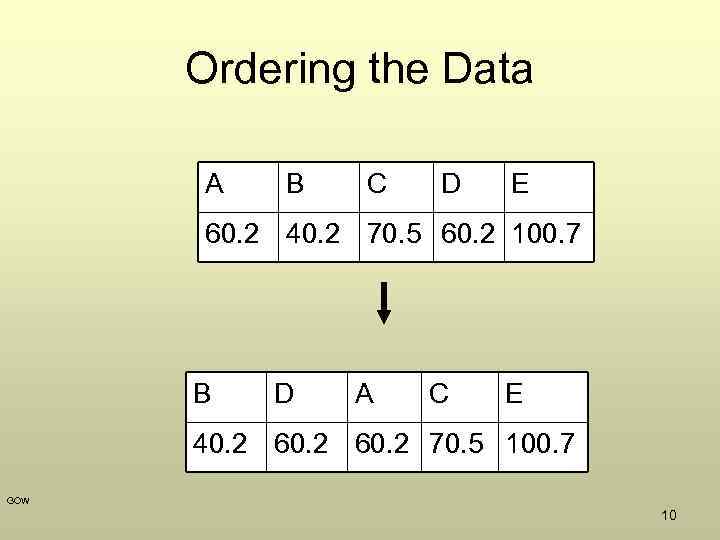Ordering the Data A B C D E 60. 2 40. 2 70. 5 60. 2 100. 7 B D A C E 40. 2 60. 2 70. 5 100. 7 GOW 10

Please, FIND the range and mean GOW

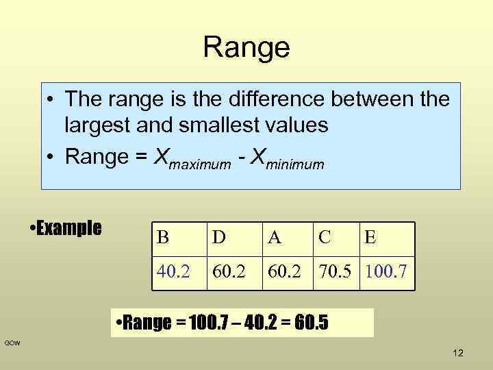Range • The range is the difference between the largest and smallest values • Range = Xmaximum - Xminimum • Example B D A C E 40. 2 60. 2 70. 5 100. 7 • Range = 100. 7 – 40. 2 = 60. 5 GOW 12

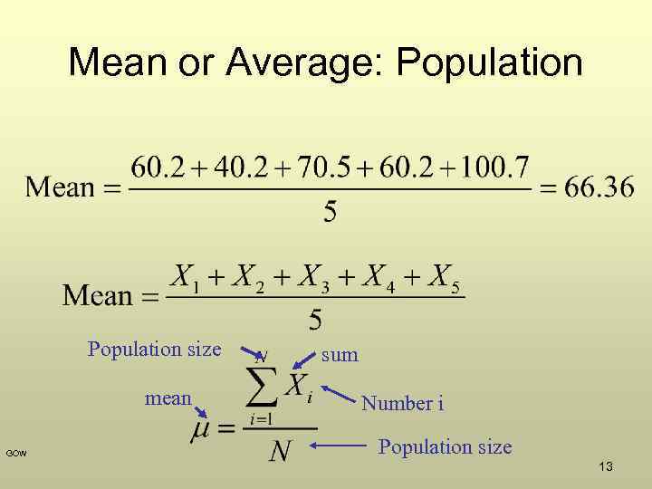Mean or Average: Population size mean GOW sum Number i Population size 13

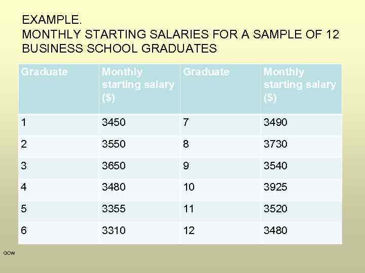EXAMPLE. MONTHLY STARTING SALARIES FOR A SAMPLE OF 12 BUSINESS SCHOOL GRADUATES Graduate Monthly starting salary ($) 1 3450 7 3490 2 3550 8 3730 3 3650 9 3540 4 3480 10 3925 5 3355 11 3520 6 GOW Monthly Graduate starting salary ($) 3310 12 3480

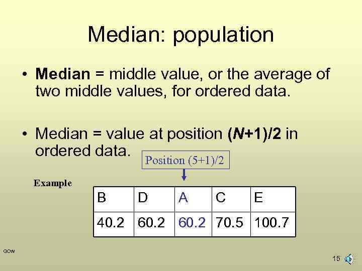Median: population • Median = middle value, or the average of two middle values, for ordered data. • Median = value at position (N+1)/2 in ordered data. Position (5+1)/2 Example B D A C E 40. 2 60. 2 70. 5 100. 7 GOW 15

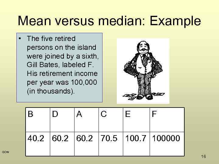Mean versus median: Example • The five retired persons on the island were joined by a sixth, Gill Bates, labeled F. His retirement income per year was 100, 000 (in thousands). B D A C E F 40. 2 60. 2 70. 5 100. 7 100000 GOW 16

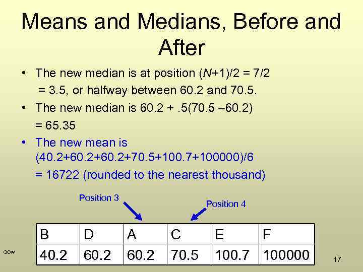Means and Medians, Before and After • The new median is at position (N+1)/2 = 7/2 = 3. 5, or halfway between 60. 2 and 70. 5. • The new median is 60. 2 +. 5(70. 5 – 60. 2) = 65. 35 • The new mean is (40. 2+60. 2+70. 5+100. 7+100000)/6 = 16722 (rounded to the nearest thousand) Position 3 GOW B 40. 2 D 60. 2 Position 4 A 60. 2 C 70. 5 E F 100. 7 100000 17

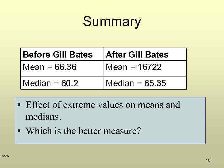Summary Before Gill Bates Mean = 66. 36 After Gill Bates Mean = 16722 Median = 60. 2 Median = 65. 35 • Effect of extreme values on means and medians. • Which is the better measure? GOW 18

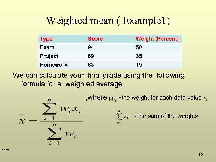Weighted mean ( Example 1) Type Score Weight (Percent) Exam 94 50 Project 89 35 Homework 83 15 We can calculate your final grade using the following formula for a weighted average , where -the weight for each data value - the sum of the weights GOW 19

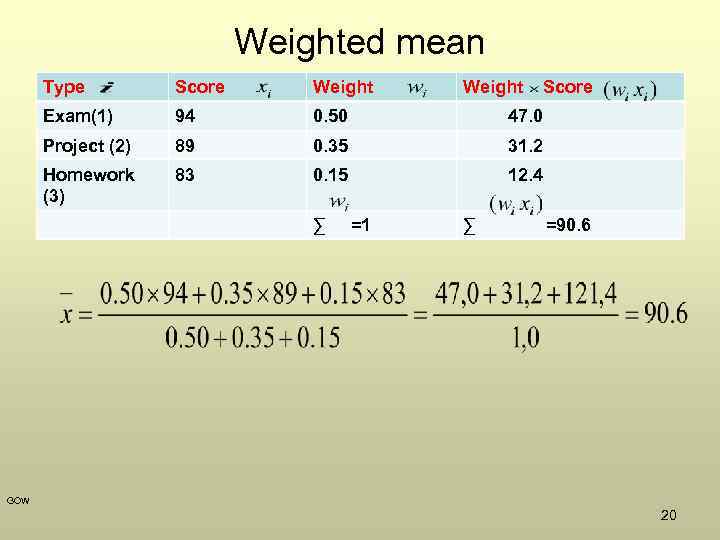Weighted mean Type Score Weight Exam(1) 94 0. 50 47. 0 Project (2) 89 0. 35 31. 2 Homework (3) 83 0. 15 12. 4 ∑ =1 Weight ∑ Score =90. 6 GOW 20

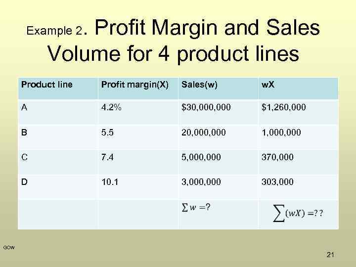. Profit Margin and Sales Volume for 4 product lines Example 2 Product line Profit margin(X) Sales(w) w. X A 4. 2% $30, 000 $1, 260, 000 B 5. 5 20, 000 1, 000 C 7. 4 5, 000 370, 000 D 10. 1 3, 000 303, 000 GOW 21

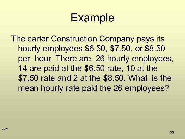Example The carter Construction Company pays its hourly employees $6. 50, $7. 50, or $8. 50 per hour. There are 26 hourly employees, 14 are paid at the $6. 50 rate, 10 at the $7. 50 rate and 2 at the $8. 50. What is the mean hourly rate paid the 26 employees? GOW 22

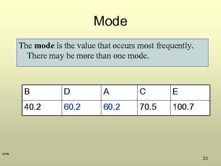Mode The mode is the value that occurs most frequently. There may be more than one mode. B D A C E 40. 2 60. 2 70. 5 100. 7 GOW 23

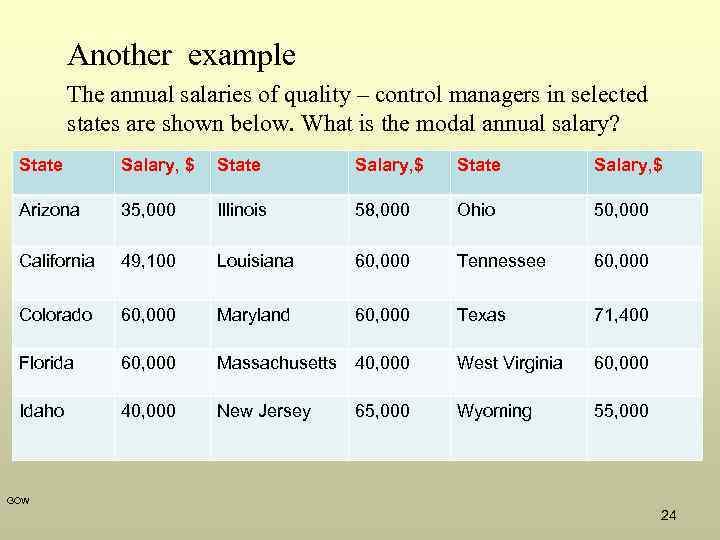Another example The annual salaries of quality – control managers in selected states are shown below. What is the modal annual salary? State Salary, $ Arizona 35, 000 Illinois 58, 000 Ohio 50, 000 California 49, 100 Louisiana 60, 000 Tennessee 60, 000 Colorado 60, 000 Maryland 60, 000 Texas 71, 400 Florida 60, 000 Massachusetts 40, 000 West Virginia 60, 000 Idaho 40, 000 New Jersey Wyoming 55, 000 65, 000 GOW 24

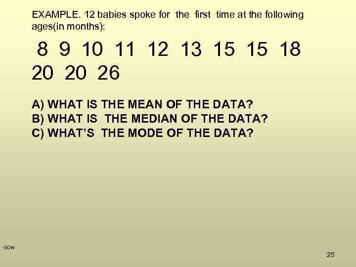EXAMPLE. 12 babies spoke for the first time at the following ages(in months): 8 9 10 11 12 13 15 15 18 20 20 26 A) WHAT IS THE MEAN OF THE DATA? B) WHAT IS THE MEDIAN OF THE DATA? C) WHAT’S THE MODE OF THE DATA? GOW 25

EXAMPLE. THE TEST SCORES OF A CLASS OF 20 STUDENTS HAS A MEAN OF 71. 6 AND THE TEST SCORES OF ANOTHER CLASS OF 14 STUDENTS HAVE A MEAN OF 78. 4. FIND THE MEAN OF THE COMBINED GROUP. EXAMPLE. EXPLAIN WHY THE CONCLUSION DRAWN IS NOT VALID. A BUSINESS WOMAN CALCULATES THE MEDIAN COST OF THE FIVE BUSINESS TRIPS THAT SHE TOOK IN A MONTH IS $600 AND CALCULATES THAT THE TOTAL COST MUST HAVE BEEN $3000 GOW 26

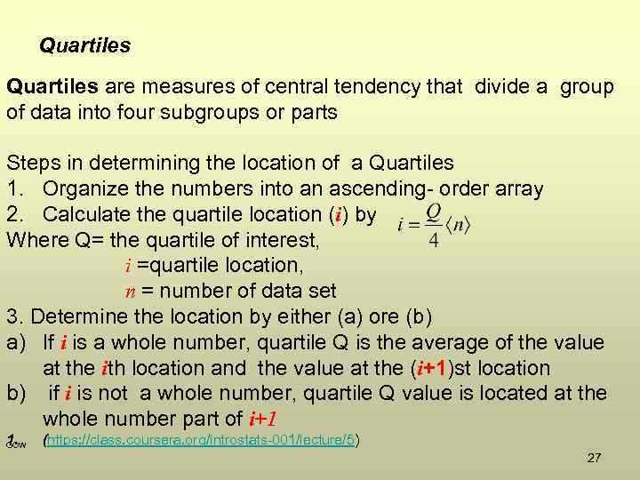Quartiles are measures of central tendency that divide a group of data into four subgroups or parts Steps in determining the location of a Quartiles 1. Organize the numbers into an ascending- order array 2. Calculate the quartile location (i) by Where Q= the quartile of interest, i =quartile location, n = number of data set 3. Determine the location by either (a) ore (b) a) If i is a whole number, quartile Q is the average of the value at the ith location and the value at the (i+1)st location b) if i is not a whole number, quartile Q value is located at the whole number part of i+1 1. GOW (https: //class. coursera. org/introstats-001/lecture/5) 27

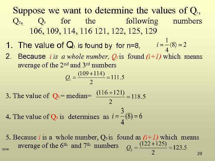Suppose we want to determine the values of Q , 1 Q 2, Q 3 for the following 106, 109, 114, 116 121, 122, 125, 129 numbers 1. The value of Q 1 is found by for n=8, 2. Because i is a whole number, Q 1 is found (i+1) which means average of the 2 nd and 3 rd numbers 3. The value of Q 2 = median= 4. The value of Q 3 is determines as 5. Because i is a whole number, Q 3 is found as (i+1) which means average of the 6 th and 7 th numbers GOW 28

Measures of Dispersion The simplest measure of dispersion is the range Range= largest value- Smallest value Another measure of variability is the interquartile range The interquartile range is the range of values between the first and third quartile Interquartile range= Q 3 -Q 1 GOW 29

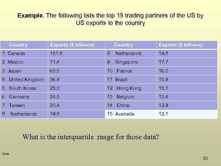Example. The following lists the top 15 trading partners of the US by US exports to the country Country Exports ($ billions) 1 Canada 151. 8 8 2 Mexico 71. 4 9 Singapore 17. 7 3 Japan 65. 5 10 France 16. 0 4 United Kingdom 36. 4 11 Brazil 15. 9 5 South Korea 25. 0 12 Hong Kong 15. 1 6 Germany 24. 5 13 Belgium 13. 4 7 Taiwan 20. 4 14 China 12. 9 8 19. 8 15 Australia 12. 1 Netherlands 19. 8 What is the interquartile range for those data? GOW 30

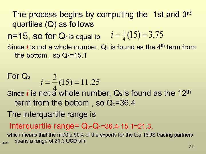The process begins by computing the 1 st and 3 rd quartiles (Q) as follows n=15, so for Q 1 is equal to Since i is not a whole number, Q 1 is found as the 4 th term from the bottom , so Q 1=15. 1 For Q 3 Since i is not a whole number, Q 3 is found as the 12 th term from the bottom , so Q 3=36. 4 The interquartile range is Interquartile range= Q 3 -Q 1=36. 4 -15. 1=21. 3, which means that the middle 50% of the exports for the top 15 US trading partners spans a range of 21. 3 USD bln GOW 31

Mean absolute deviation, Variance and Standard Deviation These are other measures of variability as follows: variance, the standard deviation and the mean absolute deviation GOW 32

Example. Suppose a small company has started a production line to build computers. During the first 5 weeks of production, the output is 5, 9, 16, 17 and 18 computers. Which descriptive statistics could the owner use to measure the early progress of production? GOW 33

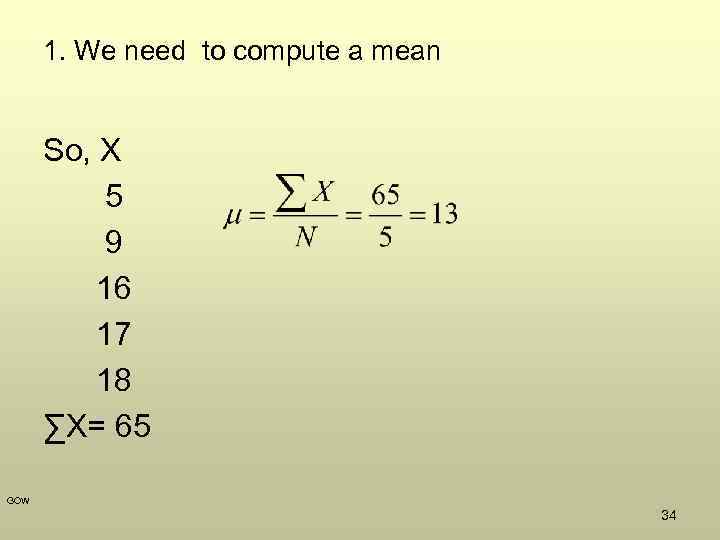1. We need to compute a mean So, X 5 9 16 17 18 ∑X= 65 GOW 34

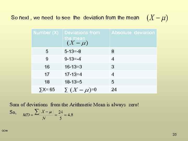So next , we need to see the deviation from the mean Number (X) Deviations from the mean Absolute deviation 5 5 -13=-8 8 9 9 -13=-4 4 16 16 -13=3 3 17 17 -13=4 4 18 18 -13=5 5 ∑ =0 24 ∑X= 65 Sum of deviations from the Arithmetic Mean is always zero! So, GOW 35

Variance and Standard deviation Variance is the arithmetic mean of the squared deviations from the mean Standard deviation is the square root of the variance GOW 36

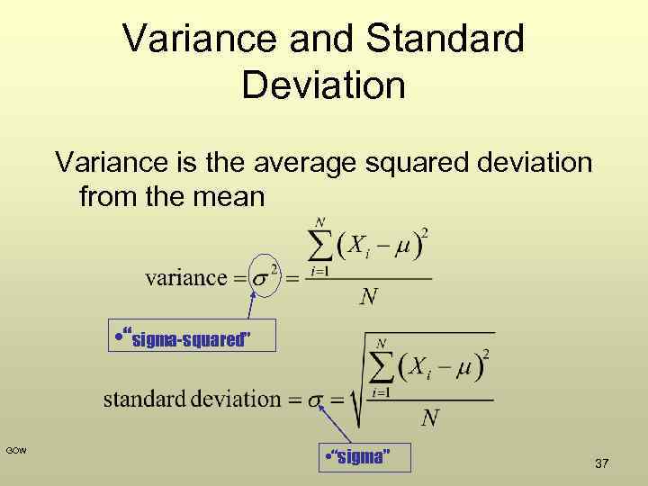Variance and Standard Deviation Variance is the average squared deviation from the mean • “sigma-squared” GOW • “sigma” 37

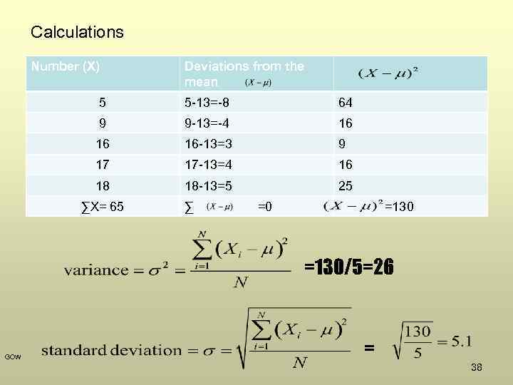Calculations Number (X) Deviations from the mean 5 5 -13=-8 64 9 9 -13=-4 16 16 16 -13=3 9 17 17 -13=4 16 18 18 -13=5 25 ∑ =0 =130 ∑X= 65 =130/5=26 GOW = 38

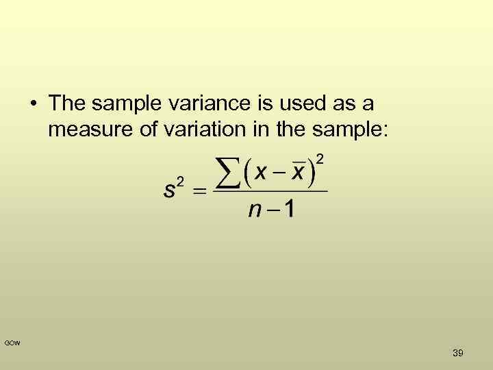• The sample variance is used as a measure of variation in the sample: GOW 39

• The purpose of calculating a sample statistic is to estimate the corresponding population parameter. • If we took many samples from a population with mean μ, calculated the sample means and then averaged these estimates, we would find that their average is very close to μ. GOW 40

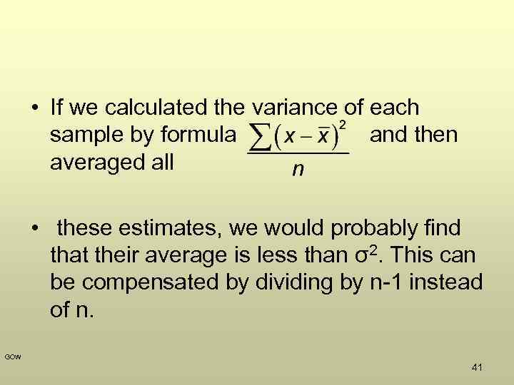• If we calculated the variance of each sample by formula and then averaged all • these estimates, we would probably find that their average is less than σ2. This can be compensated by dividing by n-1 instead of n. GOW 41

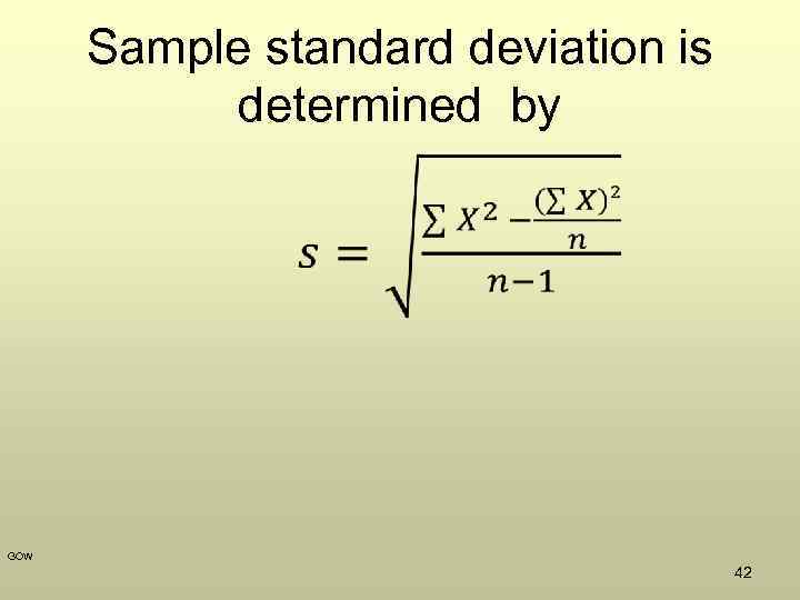Sample standard deviation is determined by • GOW 42

Variance and standard deviation are the most commonly used indicators of variation. Why ? The reasons are as follows: a) they are included in most of theorems of probability theory, and mathematical statistics b) the variance can be decomposed into components, to assess the impact of various factors contributing to the variation of feature c) variance is used to construct indicators tightness correlation, when evaluating the results of sample surveys, analysis of variance, etc. GOW 43

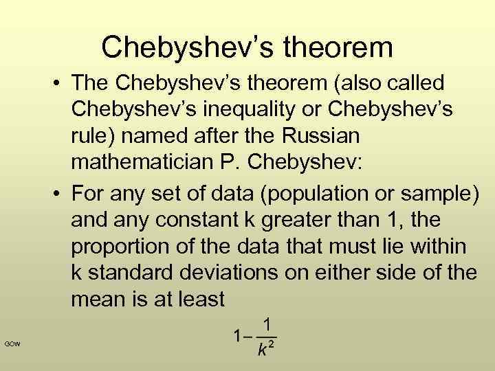
Chebyshev’s theorem • The Chebyshev’s theorem (also called Chebyshev’s inequality or Chebyshev’s rule) named after the Russian mathematician P. Chebyshev: • For any set of data (population or sample) and any constant k greater than 1, the proportion of the data that must lie within k standard deviations on either side of the mean is at least GOW

Chebyshev’s theorem • The Chebyshev’s theorem (also called Chebyshev’s inequality or Chebyshev’s rule) named after the Russian mathematician P. Chebyshev: • For any set of data (population or sample) and any constant k greater than 1, the proportion of the data that must lie within k standard deviations on either side of the mean is at least GOW

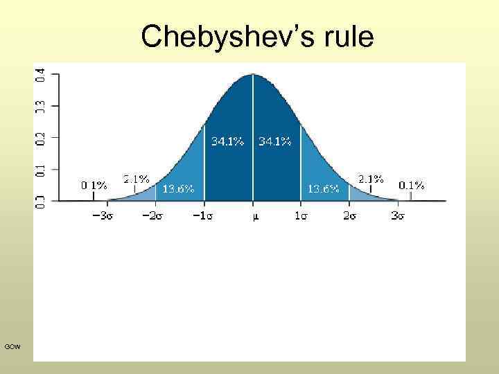
Chebyshev’s theorem • Hence, we can be sure that at least 11/(22)=3/4 or 75% of the values in any data set must lie within two standard deviations on either side of the mean. • In case of a normal distribution (we will study it later) about 95% of the values will lie within two standard deviations. GOW

Chebyshev’s rule GOW

BYE GOW 48

LECTURE 3 GOW 49

GOW 50

GOW 51

GOW 52

GOW 53

GOW 54

GOW 55

GOW 56

GOW 57

GOW 58

GOW 59

GOW 60

GOW 61

GOW 62

GOW 63

GOW 64

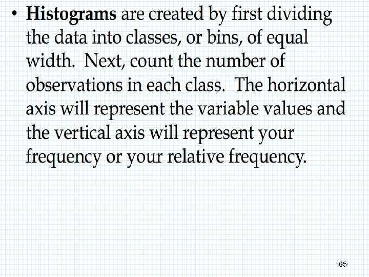GOW 65

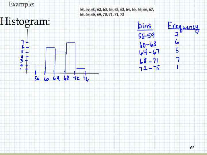GOW 66

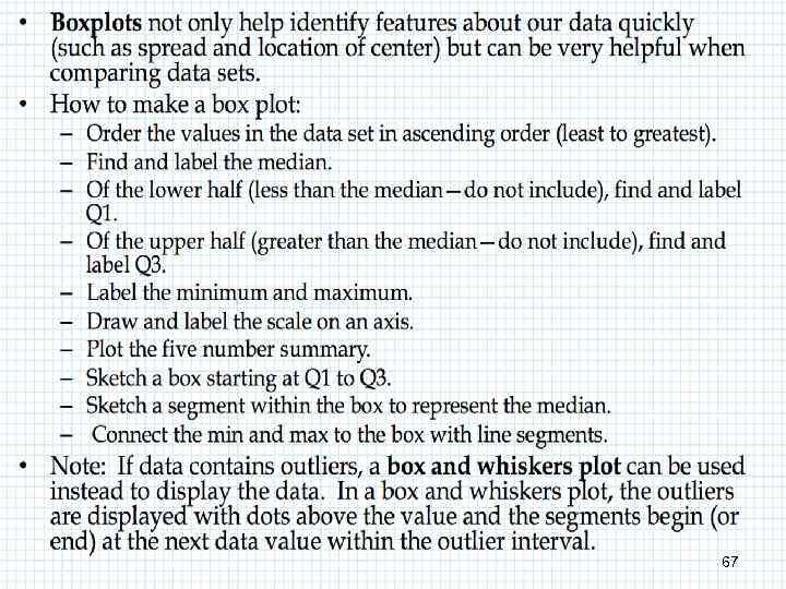GOW 67

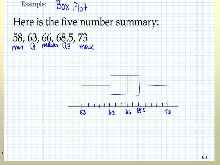GOW 68

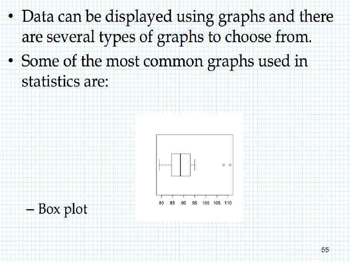
Box plots • A box plot is a convenient way of describing numerical data • Before drawing a box plot we need to get acquainted with the several notions: – The median – Quartile and interquartile range – Outliers and Tukey rule GOW

Box plots • The quartiles are three numbers that divide an ordered data set into four equal parts. The second quartile is the median. • The first quartile is the data point such that a quarter of data points lie below it • The third quartile is the data point such that a quarter of data points lie above it GOW

Box plots • Rank of quartile value=(1+median rank)/2 • You’re given data: 31, 33, 36, 37, 38, 39, 41, 44, 47. Determine the quartiles? • The median (the second quartile) is 37. 5. Its rank is 5. 5 • The rank of the quartile is (1+5)/2=3 • Hence, the first quartile is 36, the third is 41. GOW

Box plots • Interquartile range is the difference (or distance) between the first and third quartiles • 41 -36=5 • Outliers – data points which lie far away from the mean GOW

John Tukey's (1915 -2000) method considers observation Y an outlier if: • Y < (Q 1 − 1. 5 IQR) or Y > (Q 3 + 1. 5 IQR), • where Q 1 = lower quartile, Q 3 = upper quartile, and IQR = (Q 3 − Q 1) is the interquartile range. Outliers distort the average and standard deviation and make these statistics unreliable. John Tukey, Exploratory Data Analysis, Addison. Wesley, 1977, pp. 43 -44. GOW 73

Tukey rule • A step is 1. 5 multiplied by the interquartile range. • From the previous example the interquartile range is 5. The step is 7. 5 • Outliers are data points that are smaller than the first quartile minus the step or larger than the third quartile plus the step. • In the previous example the lower fence is 36 -7. 5=28. 5 and the upper fence is 41+7. 5=48. 5 GOW

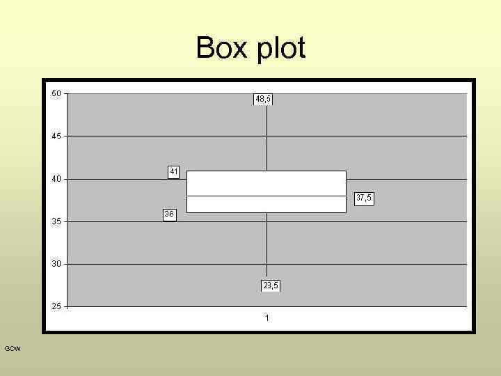
Box plots • If instead you had: 20, 33, 36, 37, 38, 39, 41, 44, 47. • The median is 37. 5. The first quartile is 36, the third is 41. • The lower fence is 36 -7. 5=28. 5 and the upper fence is 41+7. 5=48. 5. Hence the first data point (20) is an outlier GOW

Box plot GOW

Box plots GOW • Box plots show more than quartiles and outliers. They indicate the distribution’s shape – whether it is symmetric or skewed. • Symmetric – the left side of the plot (to the left of the median) is a mirror image of the right side. • Skewed distribution – the median doesn’t lie in the middle of the box. In previous example, the right side is larger. We say it is skewed to the right.

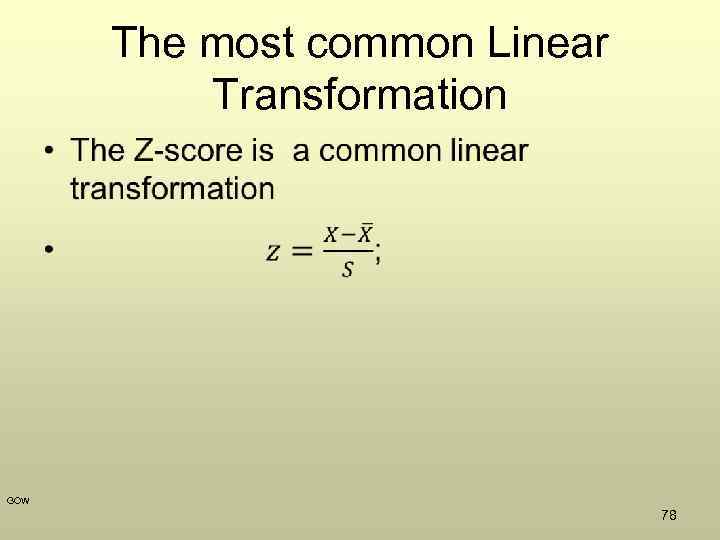The most common Linear Transformation • GOW 78

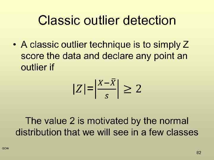
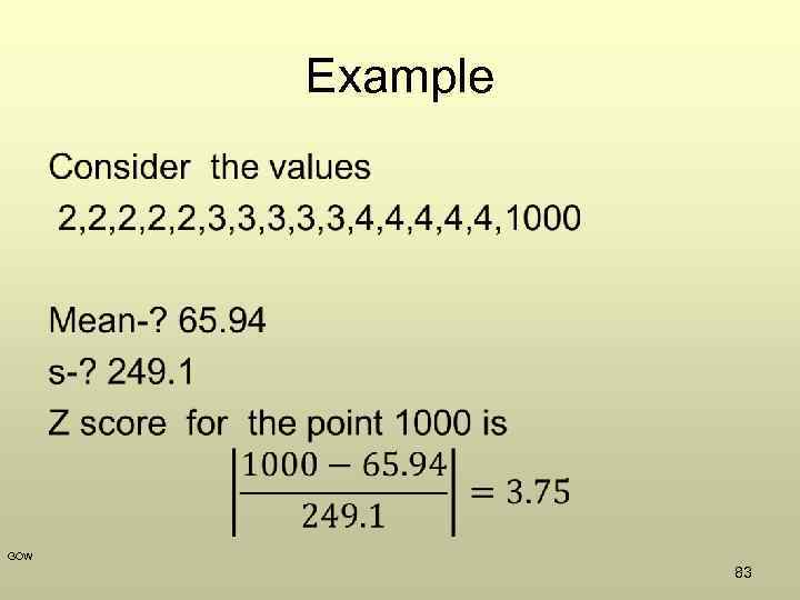
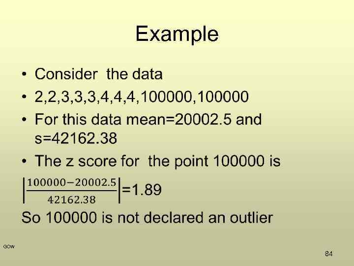
Using Z’s to compare values • Since z- scores reflect how far a score is from the mean they are a good way to standardize scores • We can take any distribution and express all values as z -scores(distances from the mean). So, no matter the scale we originally used to measure the variable, it will be expressed in a standard form. • This standard form can be used to convert different scales to the same scale so that direct comparison of values from the two different distributions can be directly compared GOW 79

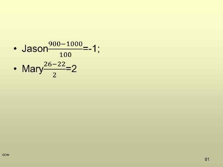
Used for comparison purposes • Mary ACT score is 26. Jason’s SAT score is 900. Who did better? • The mean SAT score is 1000 with standard deviation of 100 SAT points • The mean ACT score is 22 with standard deviation of 2 ACT points • Calculate Z- scores-? GOW 80

• GOW 81

Classic outlier detection • GOW 82

Example • GOW 83

Example • GOW 84

GOW 85

GOW 86

GOW 87

GOW 88

GOW 89

GOW 90

GOW 91

GOW 92

GOW 93

GOW 94

GOW 95

GOW 96

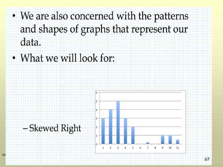GOW 97

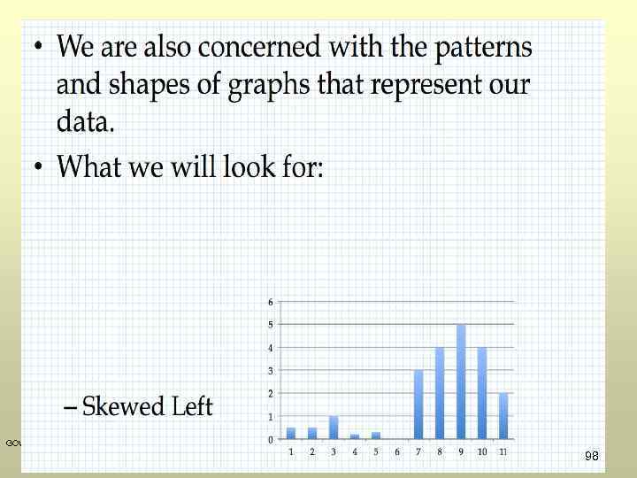GOW 98

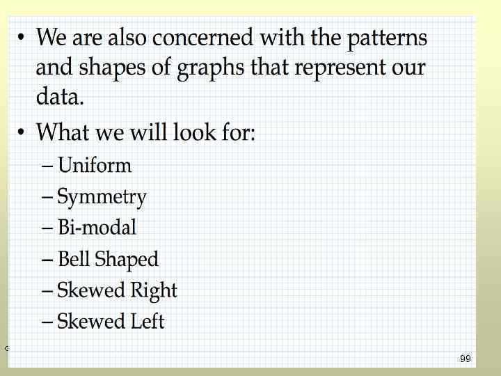GOW 99

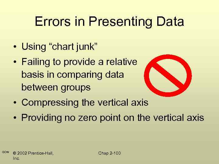Errors in Presenting Data • Using “chart junk” • Failing to provide a relative basis in comparing data between groups • Compressing the vertical axis • Providing no zero point on the vertical axis GOW © 2002 Prentice-Hall, Inc. Chap 2 -100

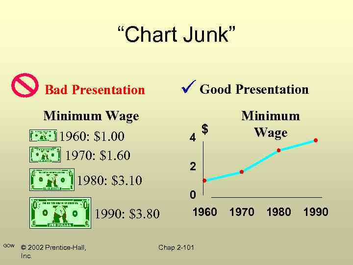“Chart Junk” Good Presentation Bad Presentation Minimum Wage 1960: $1. 00 1970: $1. 60 4 $ Minimum Wage 2 1980: $3. 10 0 1990: $3. 80 GOW © 2002 Prentice-Hall, Inc. 1960 Chap 2 -101 1970 1980 1990

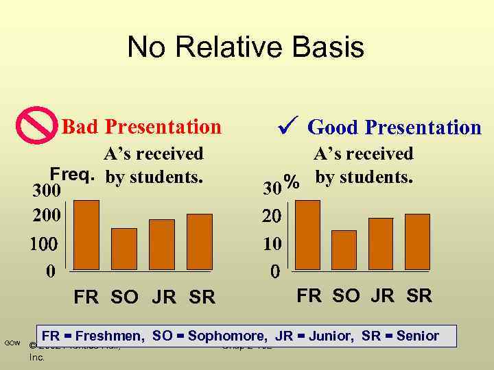No Relative Basis Bad Presentation A’s received Freq. by students. 300 200 0 FR SO JR SR GOW Good Presentation A’s received % by students. 30 10 FR SO JR SR FR = Freshmen, SO = Sophomore, JR = Junior, SR = Senior © 2002 Prentice-Hall, Inc. Chap 2 -102

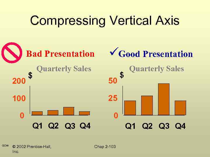Compressing Vertical Axis Bad Presentation 200 $ Good Presentation Quarterly Sales 50 100 25 0 0 Q 1 Q 2 Q 3 Q 4 GOW $ Quarterly Sales © 2002 Prentice-Hall, Inc. Q 1 Q 2 Q 3 Q 4 Chap 2 -103

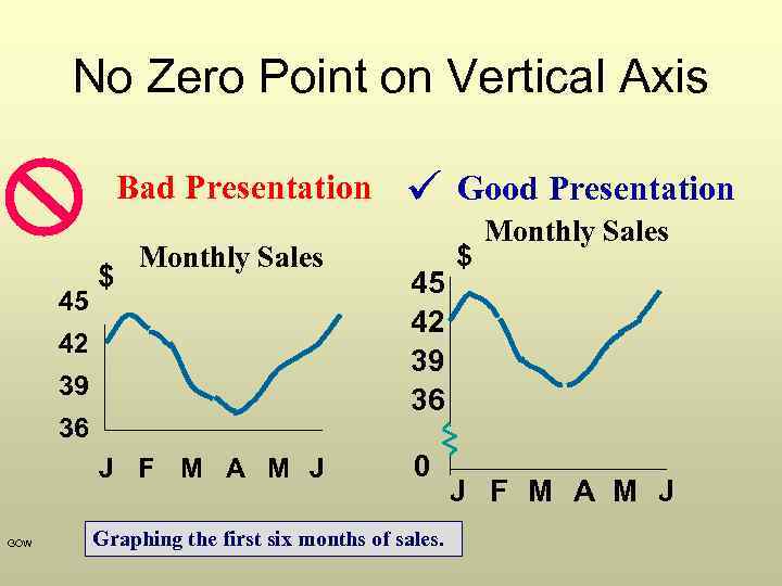No Zero Point on Vertical Axis Bad Presentation 45 $ Monthly Sales 42 39 36 J F M A M J GOW 45 42 39 36 0 Graphing the first six months of sales. Chap 2 -104 Good Presentation $ Monthly Sales J F M A M J