Lecture 2 Control on Prices Production Profits

Скачать презентацию Lecture 2 Control on Prices Production Profits

b2c935162d34a9ee852f039b0279d835.ppt

Количество слайдов: 81

Lecture 2: Control on Prices, Production & Profits Dr. Rajeev Dhawan Director Given to the EMBA 8400 Class January 5, 2008

Chapter 6 Controls on Prices

Controls on Prices ¨ Price Ceiling (e. g. rent control) – A legal maximum on the price at which a good can be sold. – If the price ceiling is set below the equilibrium price, it leads to a shortage. ¨ Price Floor (e. g. minimum wage) – A legal minimum on the price at which a good can be sold. – If the price ceiling is set above the equilibrium price, it leads to a surplus.

Price Ceiling: Beer Shortage …Rent Control Too Beer Supply Equilibrium price $3 2 Price ceiling Shortage Demand 0 75 125 Quantity supplied Quantity demanded Pints

Price Floor: Beer Surplus Price of Beer Supply Surplus Equilibrium$4 price Price floor $3 Demand 0 75 125 Quantity demanded Quantity supplied Quantity of Beer

Chapter 2 Production

Production ¨ What is production? – The activity by which we convert inputs (labor, land & capital) into goods and services ¨ What limits production? – Inputs (resources) – Technology ØGovernment interference

Circular Flow Diagram Revenue Goods and services sold MARKETS FOR GOODS AND SERVICES • Firms sell • Households buy Spending Goods and services bought HOUSEHOLDS • Buy and consume goods and services • Own and sell factors of production FIRMS • Produce and sell goods and services • Hire and use factors of production Factors of production Wages, rent, and profit Labor, land, capital MARKETS and FOR FACTORS OF PRODUCTION • Households sell • Firms buy Income = Flow of inputs and outputs = Flow of dollars

Production Possibilities Frontier ¨ Definition: the amount of goods a firm or society can produce given a fixed amount of land, labor and other inputs.

Production Possibilities Frontier Quantity of Pretzels Produced 4, 000 D 3, 000 a 2, 200 2, 100 2, 000 C E A B 1, 000 0 300 d . 600 750 b Production possibilities frontier c 1, 000 Quantity of Beer Produced

Production Function I Y (Production) = F (Inputs) Y=I Marginal Product: it is the increase in output that arises from an additional unit of input. Marginal Product (MP) = ∆ Output / ∆Input

Production Function II Y = I 2 Marginal Product (MP) = ∆ Output / ∆Input

Production Function III Y = √I Marginal Product (MP) = ∆ Output / ∆Input

Returns to Scale ¨ Returns to Scale: the property of the production function that when you double your inputs, your output either doubles, more than doubles, or less than doubles. Y=I MP ↑ IRS MP ↓ DRS Y=I 2 IRS CRS DRS Y = √I

Chapter 13 Costs & Profits

Cost of Production ¨ Cost of production includes all the opportunity costs of making the output of goods and services. – Explicit costs: input costs that require a direct outlay of money by the firm. – Implicit costs: input costs that do not require an outlay of money by the firm.

Profits ¨ The firm’s objective is to maximize profits Profit = Total revenue - Total cost ¨ Economic Profit: total revenue minus total cost, including both explicit and implicit costs. ¨ Accounting Profit: total revenue minus only the firm’s explicit costs.

How an Economist Views a Firm Profits How an Accountant Views a Firm Economic profit Accounting profit Revenue Implicit costs Explicit costs Revenue Total opportunity costs Explicit costs Copyright © 2004 South-Western

Article: Economic Profit vs. Accounting Profit WSJ; by: Robert Bartley ¨ Profit is any income to a proprietor—Marxist Labor View—which is fallacious ¨ The economist is interested in the dynamic forces of production while: The accountant is interested in proprietorship…. cost as a deduction from the owner’s income ¨ Economic profit is the unimputable income i. e. “the residium of product remaining after payment is made at rates established in competition with all comers for all services of men or things for which competition exists” ¨ The highest uses depend on economic profit-rate of return on assets-not on accounting profits. ¨ The issue of interest on equity has tended to constitute an issue between accountants and economic theorists ¨ EPS measures the corporate profit and is called the accounting profit ¨ Peter Drucker: EPS represents taxable earnings i. e. after all deductions, is purely arbitrary concept and has nothing to do with business performance ¨ NET-NET: Takes skill to convert EPS into meaningful economic profit concept.

Marginal Product ¨ Marginal Product: for any input, it is the increase in output that arises from an additional unit of that input. ¨ Diminishing Marginal Product: the marginal product of an input declines as the quantity of the input increases. Y = √I

Diminishing Marginal Product Quantity of Output (cookies per hour) Production function 150 140 130 120 110 100 90 80 70 60 50 40 30 20 10 0 1 2 3 4 5 Number of Workers Hired

Fixed & Variable Costs ¨ Fixed costs: those costs that do not vary with the quantity of output produced. ¨ Variable costs: those costs that do vary with the quantity of output produced. TC = TFC + TVC ¨ Total Costs – – Total Fixed Costs (TFC) Total Variable Costs (TVC) Total Costs (TC) TC = TFC + TVC

Total Cost Curve ¨ Shows the relationship between the quantity a firm can produce and its costs.

Total Cost Curve Quantity of Output (cookies per hour)

Marginal Cost ¨ Marginal Cost (MC): measures the increase in total cost that arises from an extra unit of production.

EMBA 2007 Tavern (Lemonade Example)

Tavern’s Total-Cost Curve Total Cost $15. 00 Total-cost curve 14. 00 13. 00 12. 00 11. 00 10. 00 9. 00 8. 00 7. 00 6. 00 5. 00 4. 00 3. 00 2. 00 1. 00 0 1 2 3 4 5 6 7 8 9 10 Quantity of Output (pints of beer per hour)

Tavern’s Total-Cost Curve Total Cost Total-cost curve $15. 00 14. 00 13. 00 12. 00 11. 00 10. 00 9. 00 8. 00 7. 00 6. 00 5. 00 4. 00 3. 00 2. 00 1. 00 0 1 2 3 4 5 6 7 Quantity of Output (glasses of lemonade per hour) 8 9 10

Average Costs ¨ Average costs can be determined by dividing the firm’s costs by the quantity of output it produces. ¨ The average cost is the cost of each typical unit of product. – ATC – AFC – AVC

Tavern’s Various Cost Curves Costs $3. 50 3. 25 3. 00 2. 75 2. 50 2. 25 MC 2. 00 1. 75 1. 50 ATC 1. 25 AVC 1. 00 0. 75 0. 50 AFC 0. 25 0 1 2 3 4 5 6 7 8 9 10 Quantity of Output (pints of beer per hour)

Returns/Economies of Scale ¨ Increasing Returns to Scale/Economies of scale (IRS): long-run average total cost falls as the quantity of output increases. ¨ Decreasing Returns to Scale/Diseconomies of scale (DRS): long-run average total cost rises as the quantity of output increases. ¨ Constant returns to scale (CRS): long-run average total cost stays the same as the quantity of output increases

Economies of Scale (P 282) Average Total Cost ATC in long run $12, 000 10, 000 Increasing returns to scale 0 Constant returns to scale 1, 000 1, 200 Decreasing returns to scale Quantity of Cars per Day

Chapter 14 Competitive Firms

Total Revenue ¨ Total Revenue: for a firm, is the selling price times the quantity sold. TR = (P Q) ¨ Total revenue is proportional to the amount of output.

Average Revenue ¨ Average Revenue: how much revenue a firm receives for the typical unit sold.

Marginal Revenue ¨ Marginal Revenue: the change in total revenue from an additional unit sold. MR = TR/ Q ¨ For competitive firms, marginal revenue equals the price of the good.

Profit Maximization ¨ Firms will produce where TR-TC is greatest MR=MC

Profit Maximization Costs and Revenue The firm maximizes profit by producing the quantity at which marginal cost equals marginal revenue. Suppose the market price is P. MC If the firm produces Q 2, marginal cost is MC 2. ATC MC 2 P = MR 1 = MR 2 AVC If the firm produces Q 1, marginal cost is MC 1 0 P = AR = MR Q 1 QMAX Q 2 Quantity

Measuring Profits Graphically Price P Firm with Profits MC ATC P = AR = MR 0 Quantity Q (profit-maximizing quantity)

Decision to Shut Down ¨ Shut Down: a short term decision to stop production (not to exit the market) – Fixed/Sunk costs are ignored ¨ Shut down if TR < VC ¨ Shut down if TR/Q < VC/Q – TR/Q = Average Revenue In equilibrium – VC/Q = Average Variable Cost P = MR ¨ Shut down if P < AVC

Decision to Shut Down Costs If P > ATC, the firm will continue to produce at a profit. Firm’s short-run supply curve MC ATC If P > AVC, firm will continue to produce in the short run. AVC Firm shuts down if P< AVC 0 Quantity

Decision to Exit ¨ Exit: a long run decision to leave the market ¨ The firm exits if the revenue it would get from producing is less than its total cost. ¨ Exit if TR < TC ¨ Exit if TR/Q < TC/Q ¨ Exit if P < ATC

Decision to Exit Costs Firm’s long-run supply curve Firm enters if P > ATC MC = long-run S ATC Firm exits if P < ATC 0 Quantity

Measuring Profits Graphically Price MC ATC P P = AR = MR Loss 0 Q (loss-minimizing quantity) Quantity

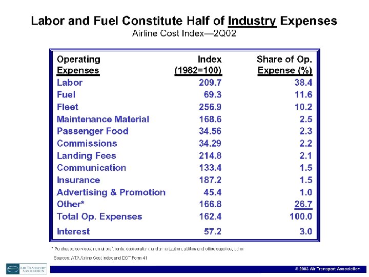
Cost & Profits Airline Industry

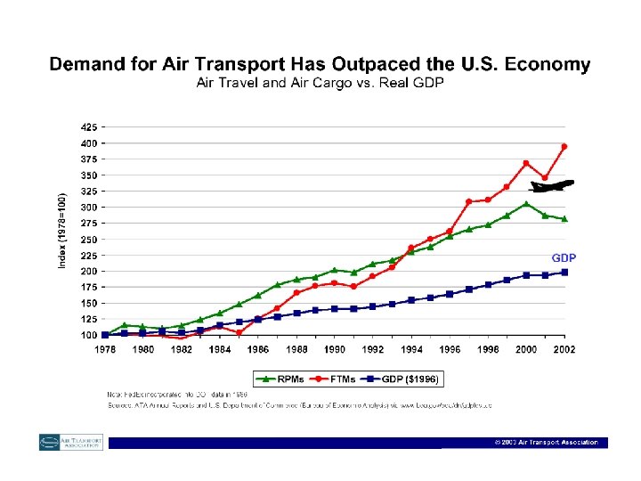
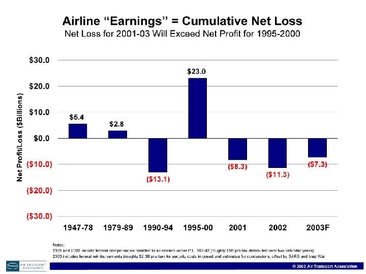
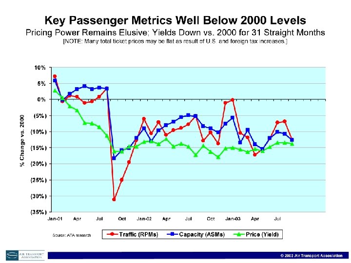
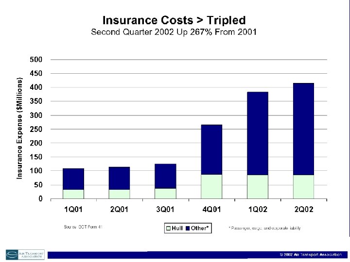
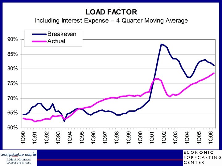
US Airline Cost Index Report 2 nd Quarter 2006

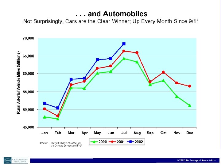
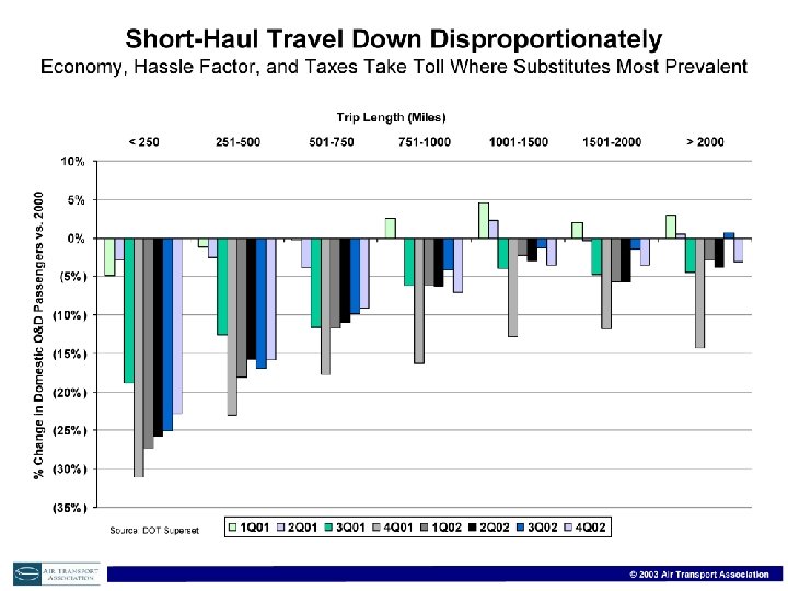
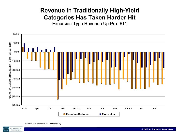
Airline Employment Down by 100, 000+ ATA 2004 Economic Report

ATA 2004 Economic Report

US Airline Cost Index Report 2 nd Quarter 2006

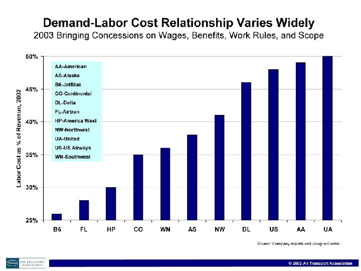
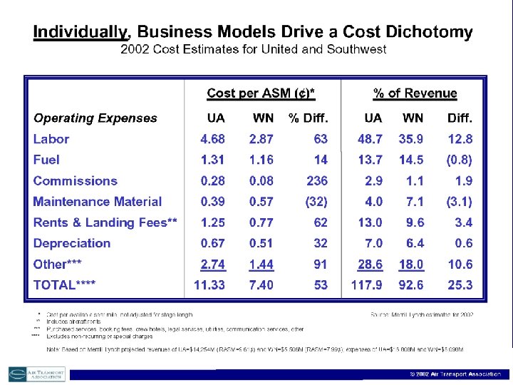
WSJ Article 2002

Article: One Airline’s Magic Time Magazine by: Sally Donnelly How does Southwest (SW) soar above its money losing rivals? ¨ Productivity Its employees work harder and are smarter, in return, they get job security and a share of profits – Pilots fly as many as 83 hours a month, compared with about 53 hours in a busy month at United Airlines – Flight attendants work almost twice as many hours as their counterparts at other airlines – Mechanics change airplane tires faster (like a NASCAR pit) and thus get higher wages than their counterparts at other airlines ¨ Flexibility – SW pilots also pitch in to help ground crews move luggage

¨ In return, SW compensates it workers in ways other than the base pay – It contributes 15% of its pre-tax income to a profit-sharing plan – It has assured all its workers and unions that there would be no lay-offs – SW doesn’t use the word “employee”, and gives them enough room to grow and learn – SW has enjoyed big savings by never having the type of defined-benefit pension plans which has proved so costly for other airlines ¨ Other advantages of SW: – Last year, SW selected 6, 000 people out of 2 million resumes received on the basis of attitudes and not necessarily skills – SW flies point-to-point domestic routes, as opposed to the complex and expensive hub-and-spoke international networks – No meals served onboard, no bulky drink carts and no entertainment – SW uses less expensive, less crowded secondary airports – Flies only one type of aircraft – Boeing 737 to reduce maintenance costs – Employees own more than 10% of SW outstanding shares, thus they work more productively and more creatively to increase their own pay checks – Lowest cost per seat mile: 7. 5 cents – Highest aircraft hours per day: 10. 9 hrs/day

So What is the Solution?

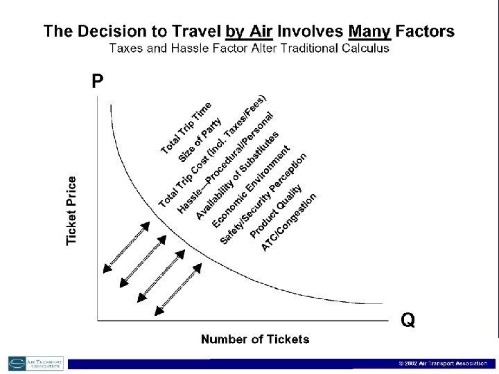
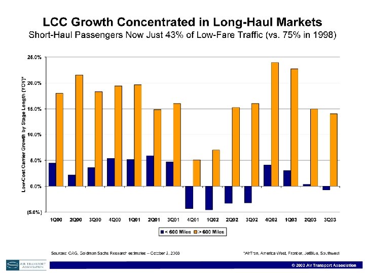
Article: The Airline Industry’s Changing Business Model ¨Do the legacy airlines have any comparative advantage that they can use in competing with their low cost rivals for domestic travelers? – The honest answer is NO. ¨The time has come for some of the airlines to either merge or liquidate so that excess capacity in the market can be reduced to profitability manage the new demand frontier. (permanent downward shift in demand curve esp. domestic flying) ¨But will the mergers or liquidations save the big boys? Maybe… ¨The only way out is a radical shift in thinking by the big airlines: outsource to low-cost airlines and allow them to bring passengers to your legacy hubs! Then fly these travelers to international destinations on your planes at premium prices where there is no competition from South-West and upstart airlines.