b737f43b7002f27c4cc733595d8e92b5.ppt
- Количество слайдов: 29
Lecture 2: Benchmarks, Performance Metrics, Cost, Instruction Set Architecture Professor Alvin R. Lebeck Compsci 220 / ECE 252 Fall 2004
Administrative • Read Chapter 3, Wulf, transmeta • Homework #1 Due September 7 – Simple scalar, read some of the documentation first – See web page for details – Questions, contact Shobana (shobana@cs. duke. edu) © 2004 Lebeck, Sorin, Roth, Hill, Wood, Sohi, Smith, Vijaykumar, Lipasti, Katz 2
Review: Trends • Technology trends are one driving force in architectural innovation • Moore’s Law • Chip Area Reachable in one clock • Power Density © 2004 Lebeck, Sorin, Roth, Hill, Wood, Sohi, Smith, Vijaykumar, Lipasti, Katz 3
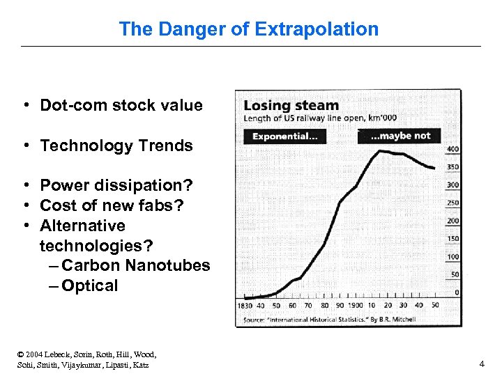
The Danger of Extrapolation • Dot-com stock value • Technology Trends • Power dissipation? • Cost of new fabs? • Alternative technologies? – Carbon Nanotubes – Optical © 2004 Lebeck, Sorin, Roth, Hill, Wood, Sohi, Smith, Vijaykumar, Lipasti, Katz 4
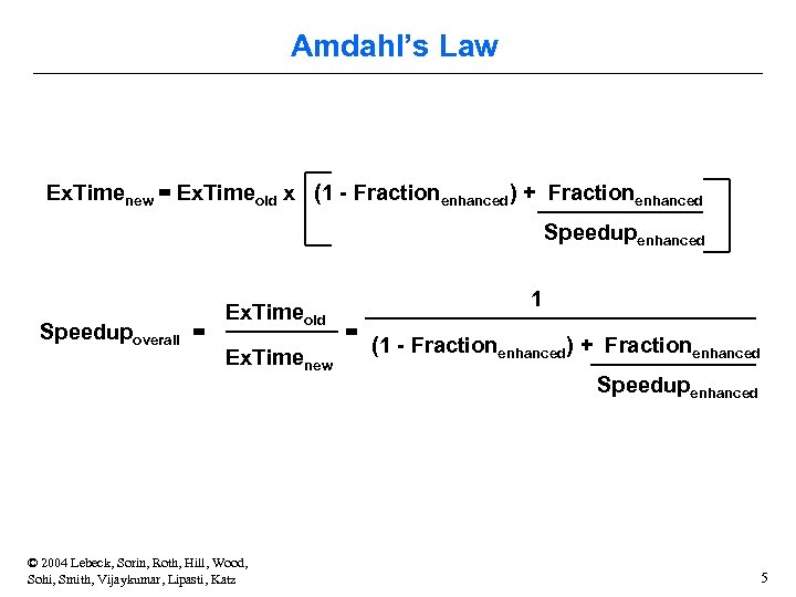
Amdahl’s Law Ex. Timenew = Ex. Timeold x (1 - Fractionenhanced) + Fractionenhanced Speedupoverall = Ex. Timeold Ex. Timenew © 2004 Lebeck, Sorin, Roth, Hill, Wood, Sohi, Smith, Vijaykumar, Lipasti, Katz 1 = (1 - Fractionenhanced) + Fractionenhanced Speedupenhanced 5
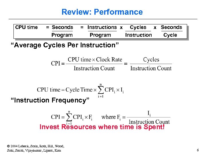
Review: Performance CPU time = Seconds = Instructions x Cycles Program Instruction Program x Seconds Cycle “Average Cycles Per Instruction” “Instruction Frequency” Invest Resources where time is Spent! © 2004 Lebeck, Sorin, Roth, Hill, Wood, Sohi, Smith, Vijaykumar, Lipasti, Katz 6
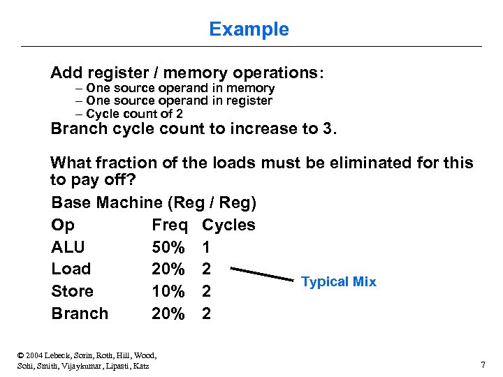
Example Add register / memory operations: – One source operand in memory – One source operand in register – Cycle count of 2 Branch cycle count to increase to 3. What fraction of the loads must be eliminated for this to pay off? Base Machine (Reg / Reg) Op Freq Cycles ALU 50% 1 Load 20% 2 Typical Mix Store 10% 2 Branch 20% 2 © 2004 Lebeck, Sorin, Roth, Hill, Wood, Sohi, Smith, Vijaykumar, Lipasti, Katz 7
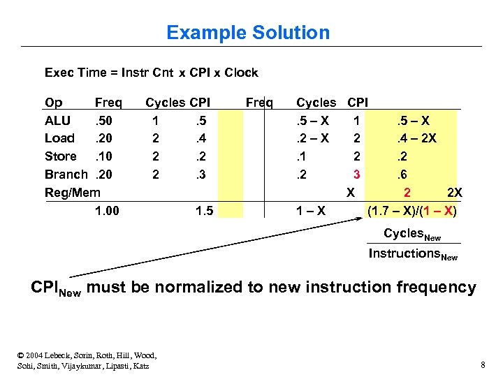
Example Solution Exec Time = Instr Cnt x CPI x Clock Op Freq ALU. 50 Load. 20 Store. 10 Branch. 20 Reg/Mem 1. 00 Cycles CPI 1. 5 2. 4 2. 2 2. 3 1. 5 Freq Cycles CPI. 5 – X 1. 5 – X. 2 – X 2. 4 – 2 X. 1 2. 2. 2 3. 6 X 2 2 X 1–X (1. 7 – X)/(1 – X) Cycles. New Instructions. New CPINew must be normalized to new instruction frequency © 2004 Lebeck, Sorin, Roth, Hill, Wood, Sohi, Smith, Vijaykumar, Lipasti, Katz 8
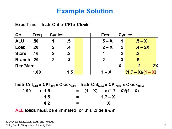
Example Solution Exec Time = Instr Cnt x CPI x Clock Op Freq ALU. 50 Load. 20 Store. 10 Branch. 20 Reg/Mem 1. 00 Cycles 1 2 2 2 . 5. 4. 2. 3 Freq. 5 – X. 2 – X. 1. 2 1. 5 1–X Cycles 1. 5 – X 2. 4 – 2 X 2. 2 3. 6 X 2 2 X (1. 7 – X)/(1 – X) Instr Cnt. Old x CPIOld x Clock. Old = Instr Cnt. New x CPINew x Clock. New 1. 00 x 1. 5 = (1 – X) x (1. 7 – X)/(1 – X) 1. 5 = 1. 7 – X 0. 2 = X ALL loads must be eliminated for this to be a win! © 2004 Lebeck, Sorin, Roth, Hill, Wood, Sohi, Smith, Vijaykumar, Lipasti, Katz 9
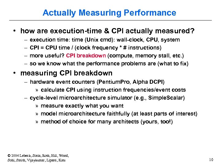
Actually Measuring Performance • how are execution-time & CPI actually measured? – – execution time: time (Unix cmd): wall-clock, CPU, system CPI = CPU time / (clock frequency * # instructions) more useful? CPI breakdown (compute, memory stall, etc. ) so we know what the performance problems are (what to fix) • measuring CPI breakdown – hardware event counters (Pentium. Pro, Alpha DCPI) » calculate CPI using instruction frequencies/event costs – cycle-level microarchitecture simulator (e. g. , Simple. Scalar) » measure exactly what you want » model microarchitecture faithfully (at least parts of interest) » method of choice for many architects (yours, too!) © 2004 Lebeck, Sorin, Roth, Hill, Wood, Sohi, Smith, Vijaykumar, Lipasti, Katz 10
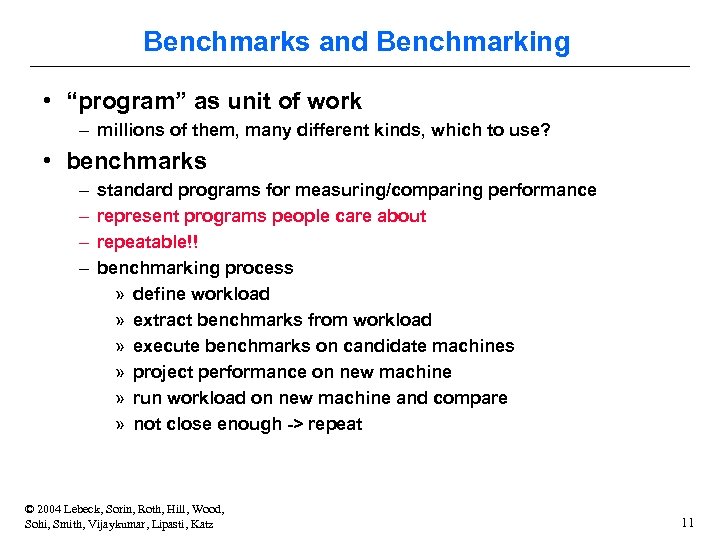
Benchmarks and Benchmarking • “program” as unit of work – millions of them, many different kinds, which to use? • benchmarks – – standard programs for measuring/comparing performance represent programs people care about repeatable!! benchmarking process » define workload » extract benchmarks from workload » execute benchmarks on candidate machines » project performance on new machine » run workload on new machine and compare » not close enough -> repeat © 2004 Lebeck, Sorin, Roth, Hill, Wood, Sohi, Smith, Vijaykumar, Lipasti, Katz 11
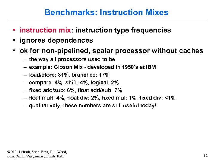
Benchmarks: Instruction Mixes • instruction mix: instruction type frequencies • ignores dependences • ok for non-pipelined, scalar processor without caches – – – – the way all processors used to be example: Gibson Mix - developed in 1950’s at IBM load/store: 31%, branches: 17% compare: 4%, shift: 4%, logical: 2% fixed add/sub: 6%, float add/sub: 7% float mult: 4%, float div: 2%, fixed mul: 1%, fixed div: <1% qualitatively, these numbers are still useful today! © 2004 Lebeck, Sorin, Roth, Hill, Wood, Sohi, Smith, Vijaykumar, Lipasti, Katz 12
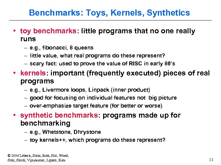
Benchmarks: Toys, Kernels, Synthetics • toy benchmarks: little programs that no one really runs – e. g. , fibonacci, 8 queens – little value, what real programs do these represent? – scary fact: used to prove the value of RISC in early 80’s • kernels: important (frequently executed) pieces of real programs – e. g. , Livermore loops, Linpack (inner product) – good for focusing on individual features not big picture – over-emphasize target feature (for better or worse) • synthetic benchmarks: programs made up for benchmarking – e. g. , Whetstone, Dhrystone – toy kernels++, which programs do these represent? © 2004 Lebeck, Sorin, Roth, Hill, Wood, Sohi, Smith, Vijaykumar, Lipasti, Katz 13
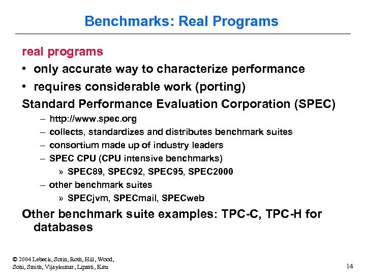
Benchmarks: Real Programs real programs • only accurate way to characterize performance • requires considerable work (porting) Standard Performance Evaluation Corporation (SPEC) – – http: //www. spec. org collects, standardizes and distributes benchmark suites consortium made up of industry leaders SPEC CPU (CPU intensive benchmarks) » SPEC 89, SPEC 92, SPEC 95, SPEC 2000 – other benchmark suites » SPECjvm, SPECmail, SPECweb Other benchmark suite examples: TPC-C, TPC-H for databases © 2004 Lebeck, Sorin, Roth, Hill, Wood, Sohi, Smith, Vijaykumar, Lipasti, Katz 14
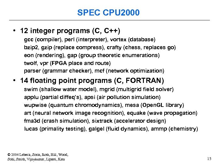
SPEC CPU 2000 • 12 integer programs (C, C++) gcc (compiler), perl (interpreter), vortex (database) bzip 2, gzip (replace compress), crafty (chess, replaces go) eon (rendering), gap (group theoretic enumerations) twolf, vpr (FPGA place and route) parser (grammar checker), mcf (network optimization) • 14 floating point programs (C, FORTRAN) swim (shallow water model), mgrid (multigrid field solver) applu (partial diffeq’s), apsi (air pollution simulation) wupwise (quantum chromodynamics), mesa (Open. GL library) art (neural network image recognition), equake (wave propagation) fma 3 d (crash simulation), sixtrack (accelerator design) lucas (primality testing), galgel (fluid dynamics), ammp (chemistry) © 2004 Lebeck, Sorin, Roth, Hill, Wood, Sohi, Smith, Vijaykumar, Lipasti, Katz 15
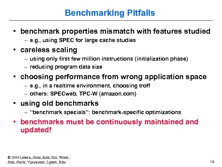
Benchmarking Pitfalls • benchmark properties mismatch with features studied – e. g. , using SPEC for large cache studies • careless scaling – using only first few million instructions (initialization phase) – reducing program data size • choosing performance from wrong application space – e. g. , in a realtime environment, choosing troff – others: SPECweb, TPC-W (amazon. com) • using old benchmarks – “benchmark specials”: benchmark-specific optimizations • benchmarks must be continuously maintained and updated! © 2004 Lebeck, Sorin, Roth, Hill, Wood, Sohi, Smith, Vijaykumar, Lipasti, Katz 16
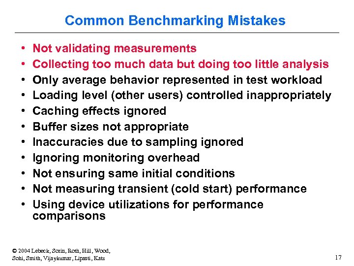
Common Benchmarking Mistakes • • • Not validating measurements Collecting too much data but doing too little analysis Only average behavior represented in test workload Loading level (other users) controlled inappropriately Caching effects ignored Buffer sizes not appropriate Inaccuracies due to sampling ignored Ignoring monitoring overhead Not ensuring same initial conditions Not measuring transient (cold start) performance Using device utilizations for performance comparisons © 2004 Lebeck, Sorin, Roth, Hill, Wood, Sohi, Smith, Vijaykumar, Lipasti, Katz 17
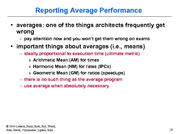
Reporting Average Performance • averages: one of the things architects frequently get wrong – pay attention now and you won’t get them wrong on exams • important things about averages (i. e. , means) – ideally proportional to execution time (ultimate metric) » Arithmetic Mean (AM) for times » Harmonic Mean (HM) for rates (IPCs) » Geometric Mean (GM) for ratios (speedups) – there is no such thing as the average program – use average when absolutely necessary © 2004 Lebeck, Sorin, Roth, Hill, Wood, Sohi, Smith, Vijaykumar, Lipasti, Katz 18
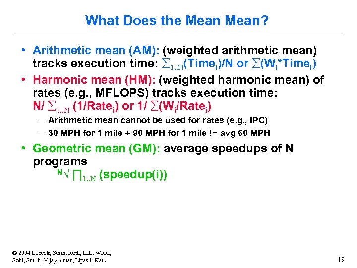
What Does the Mean? • Arithmetic mean (AM): (weighted arithmetic mean) tracks execution time: å 1. . N(Timei)/N or å(Wi*Timei) • Harmonic mean (HM): (weighted harmonic mean) of rates (e. g. , MFLOPS) tracks execution time: N/ å 1. . N (1/Ratei) or 1/ å(Wi/Ratei) – Arithmetic mean cannot be used for rates (e. g. , IPC) – 30 MPH for 1 mile + 90 MPH for 1 mile != avg 60 MPH • Geometric mean (GM): average speedups of N programs N√ ∏ 1. . N (speedup(i)) © 2004 Lebeck, Sorin, Roth, Hill, Wood, Sohi, Smith, Vijaykumar, Lipasti, Katz 19
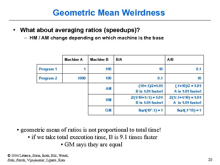
Geometric Mean Weirdness • What about averaging ratios (speedups)? – HM / AM change depending on which machine is the base Machine A Machine B B/A A/B Program 1 1 100 10 0. 1 Program 2 1000 100 0. 1 10 AM (10+. 1)/2=5. 05 B is 5. 05 faster! (. 1+10)/2 = 5. 05 A is 5. 05 faster! HM 2/(1/10+1/. 1) = 5. 05 B is 5. 05 faster! 2/(1/. 1+1/10) = 5. 05 A is 5. 05 faster! GM Sqrt(10*. 1) = 1 Sqrt(. 1*10) = 1 • geometric mean of ratios is not proportional to total time! • if we take total execution time, B is 9. 1 times faster • GM says they are equal © 2004 Lebeck, Sorin, Roth, Hill, Wood, Sohi, Smith, Vijaykumar, Lipasti, Katz 20
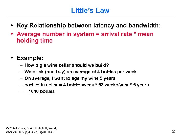
Little’s Law • Key Relationship between latency and bandwidth: • Average number in system = arrival rate * mean holding time • Example: – – – How big a wine cellar should we build? We drink (and buy) an average of 4 bottles per week On average, I want to age my wine 5 years bottles in cellar = 4 bottles/week * 52 weeks/year * 5 years = 1040 bottles © 2004 Lebeck, Sorin, Roth, Hill, Wood, Sohi, Smith, Vijaykumar, Lipasti, Katz 21
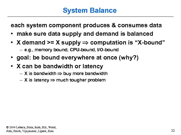
System Balance each system component produces & consumes data • make sure data supply and demand is balanced • X demand >= X supply computation is “X-bound” – e. g. , memory bound, CPU-bound, I/O-bound • goal: be bound everywhere at once (why? ) • X can be bandwidth or latency – X is bandwidth buy more bandwidth – X is latency much tougher problem © 2004 Lebeck, Sorin, Roth, Hill, Wood, Sohi, Smith, Vijaykumar, Lipasti, Katz 22
Tradeoffs “Bandwidth problems can be solved with money. Latency problems are harder, because the speed of light is fixed and you can’t bribe God” –David Clark (MIT) well. . . • can convert some latency problems to bandwidth problems • solve those with money • the famous “bandwidth/latency tradeoff” • architecture is the art of making tradeoffs © 2004 Lebeck, Sorin, Roth, Hill, Wood, Sohi, Smith, Vijaykumar, Lipasti, Katz 23
Bursty Behavior • Q: to sustain 2 IPC. . . how many instructions should processor be able to – fetch per cycle? – execute per cycle? – complete per cycle? • A: NOT 2 (more than 2) – dependences will cause stalls (under-utilization) – if desired performance is X, peak performance must be > X • programs don’t always obey “average” behavior – can’t design processor only to handle average behvaior © 2004 Lebeck, Sorin, Roth, Hill, Wood, Sohi, Smith, Vijaykumar, Lipasti, Katz 24
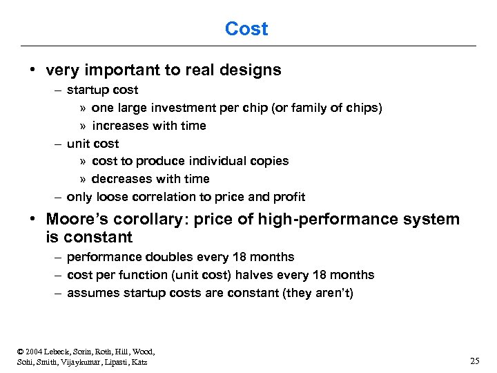
Cost • very important to real designs – startup cost » one large investment per chip (or family of chips) » increases with time – unit cost » cost to produce individual copies » decreases with time – only loose correlation to price and profit • Moore’s corollary: price of high-performance system is constant – performance doubles every 18 months – cost per function (unit cost) halves every 18 months – assumes startup costs are constant (they aren’t) © 2004 Lebeck, Sorin, Roth, Hill, Wood, Sohi, Smith, Vijaykumar, Lipasti, Katz 25
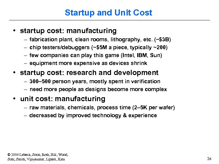
Startup and Unit Cost • startup cost: manufacturing – – fabrication plant, clean rooms, lithography, etc. (~$3 B) chip testers/debuggers (~$5 M a piece, typically ~200) few companies can play this game (Intel, IBM, Sun) equipment more expensive as devices shrink • startup cost: research and development – 300– 500 person years, mostly spent in verification – need more people as designs become more complex • unit cost: manufacturing – raw materials, chemicals, process time (2– 5 K per wafer) – decreased by improved technology & experience © 2004 Lebeck, Sorin, Roth, Hill, Wood, Sohi, Smith, Vijaykumar, Lipasti, Katz 26
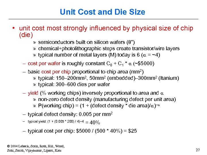
Unit Cost and Die Size • unit cost most strongly influenced by physical size of chip (die) » semiconductors built on silicon wafers (8”) » chemical+photolithographic steps create transistor/wire layers » typical number of metal layers (M) today is 6 (a = ~4) – cost per wafer is roughly constant C 0 + C 1 * a (~$5000) – basic cost per chip proportional to chip area (mm 2) » typical: 150– 200 mm 2, 50 mm 2 (embedded)– 300 mm 2 (Itanium) » typical: 300– 600 dies per wafer – yield (% working chips) inversely proportional to area and a » non-zero defect density (manufacturing defect per unit area) » P(working chip) = (1 + (defect density * die area)/a)–a – typical defect density: 0. 005 per mm 2 – typical yield: (1 + (0. 005 * 200) / 4)– 4 = 40% – typical cost per chip: $5000 / (500 * 40%) = $25 © 2004 Lebeck, Sorin, Roth, Hill, Wood, Sohi, Smith, Vijaykumar, Lipasti, Katz 27
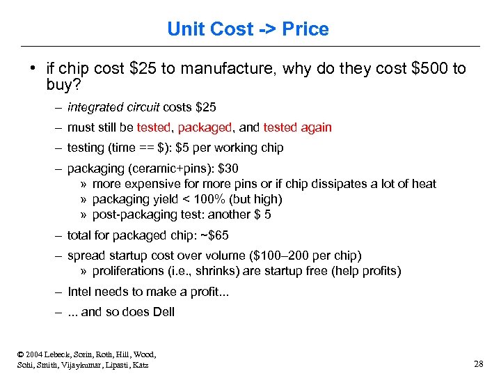
Unit Cost -> Price • if chip cost $25 to manufacture, why do they cost $500 to buy? – integrated circuit costs $25 – must still be tested, packaged, and tested again – testing (time == $): $5 per working chip – packaging (ceramic+pins): $30 » more expensive for more pins or if chip dissipates a lot of heat » packaging yield < 100% (but high) » post-packaging test: another $ 5 – total for packaged chip: ~$65 – spread startup cost over volume ($100– 200 per chip) » proliferations (i. e. , shrinks) are startup free (help profits) – Intel needs to make a profit. . . –. . . and so does Dell © 2004 Lebeck, Sorin, Roth, Hill, Wood, Sohi, Smith, Vijaykumar, Lipasti, Katz 28
Reading Summary: Performance • H&P Chapter 1 • Next Instruction Sets © 2004 Lebeck, Sorin, Roth, Hill, Wood, Sohi, Smith, Vijaykumar, Lipasti, Katz 29
b737f43b7002f27c4cc733595d8e92b5.ppt