Lecture 2 Basic Microeconomics I Dr Rajeev Dhawan

Lecture 2: Basic Microeconomics I Dr. Rajeev Dhawan Director Given to the EMBA 8400 Class March 20, 2010

Review of Last Week ¨ 10 Principles of Economics ¨ Sunk/Fixed costs ¨ Opportunity Cost and Comparative Advantage ¨ Demand Supply ¨ Price Controls

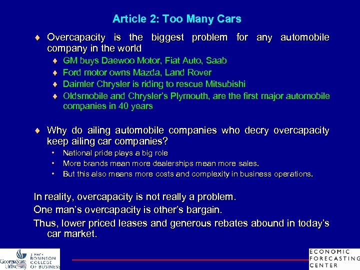
Article 2: Too Many Cars ¨ Overcapacity is the biggest problem for any automobile company in the world ¨ ¨ GM buys Daewoo Motor, Fiat Auto, Saab Ford motor owns Mazda, Land Rover Daimler Chrysler is riding to rescue Mitsubishi Oldsmobile and Chrysler’s Plymouth, are the first major automobile companies in 40 years ¨ Why do ailing automobile companies who decry overcapacity keep ailing car companies? • • • National pride plays a big role More brands mean more dealerships mean more sales. But this also means more costs and complexity in business operations. In reality, overcapacity is not really a problem. One man’s overcapacity is other’s bargain. Thus, lower priced leases and generous rebates abound in today’s car market.

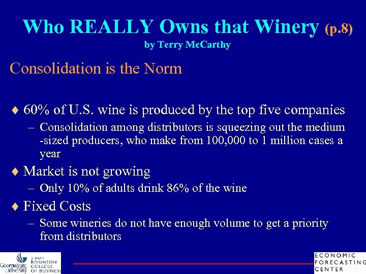
Who REALLY Owns that Winery (p. 8) by Terry Mc. Carthy Consolidation is the Norm ¨ 60% of U. S. wine is produced by the top five companies – Consolidation among distributors is squeezing out the medium -sized producers, who make from 100, 000 to 1 million cases a year ¨ Market is not growing – Only 10% of adults drink 86% of the wine ¨ Fixed Costs – Some wineries do not have enough volume to get a priority from distributors

Chapter 3 Comparative Advantage & Trade

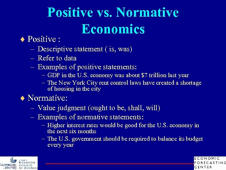
Positive vs. Normative Economics ¨ Positive : – Descriptive statement ( is, was) – Refer to data – Examples of positive statements: – GDP in the U. S. economy was about $7 trillion last year – The New York City rent control laws have created a shortage of housing in the city ¨ Normative: – Value judgment (ought to be, shall, will) – Examples of normative statements: – Higher interest rates would be good for the U. S. economy in the next six months – The U. S. government should be required to balance its budget every year

Production Possibilities Frontier ¨ The classic tale of the farmer and the rancher…or a better example if you have one. ¨ What should each produce? ¨ Why should they trade?

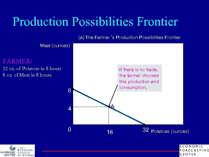
Production Possibilities Frontier (a) The Farmer ’s Production Possibilities Frontier Meat (ounces) FARMER: 32 oz. of Potatoes in 8 hours 8 oz. of Meat in 8 hours If there is no trade, the farmer chooses this production and consumption. 8 4 A 0 16 32 Potatoes (ounces)

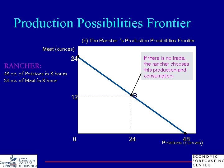
Production Possibilities Frontier (b) The Rancher ’s Production Possibilities Frontier Meat (ounces) RANCHER: 24 If there is no trade, the rancher chooses this production and consumption. 48 oz. of Potatoes in 8 hours 24 oz. of Meat in 8 hour 12 B 0 24 48 Potatoes (ounces)

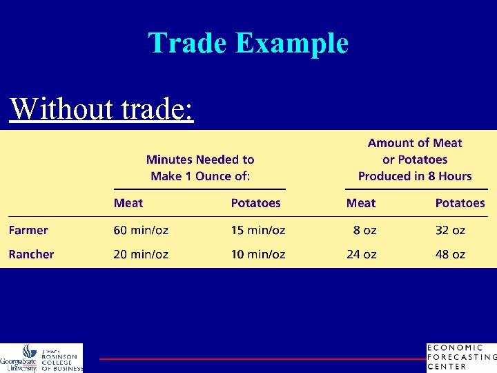
Trade Example Without trade:

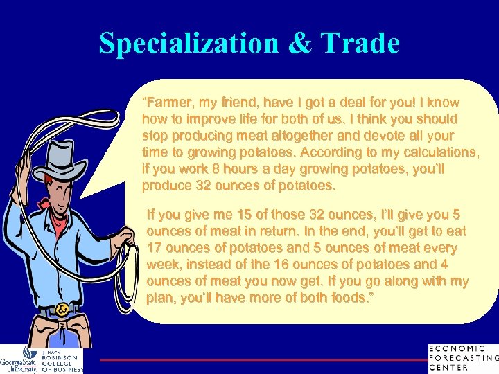
Specialization & Trade “Farmer, my friend, have I got a deal for you! I know how to improve life for both of us. I think you should stop producing meat altogether and devote all your time to growing potatoes. According to my calculations, if you work 8 hours a day growing potatoes, you’ll produce 32 ounces of potatoes. If you give me 15 of those 32 ounces, I’ll give you 5 ounces of meat in return. In the end, you’ll get to eat 17 ounces of potatoes and 5 ounces of meat every week, instead of the 16 ounces of potatoes and 4 ounces of meat you now get. If you go along with my plan, you’ll have more of both foods. ”

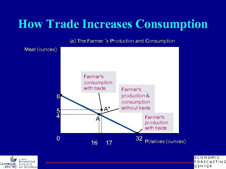
How Trade Increases Consumption (a) The Farmer ’s Production and Consumption Meat (ounces) Farmer's consumption with trade 8 5 4 0 A* Farmer's production & consumption without trade Farmer's production with trade A 16 17 32 Potatoes (ounces)

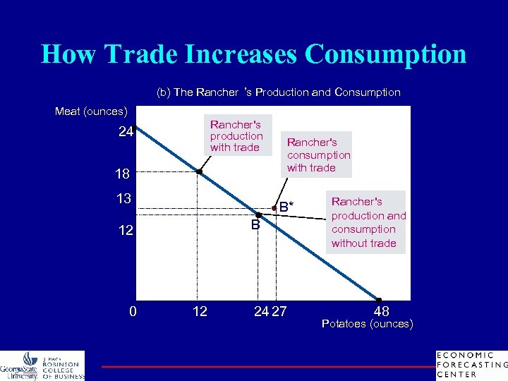
How Trade Increases Consumption (b) The Rancher ’s Production and Consumption Meat (ounces) Rancher's production with trade 24 18 13 B* B 12 0 Rancher's consumption with trade 12 24 27 Rancher's production and consumption without trade 48 Potatoes (ounces)

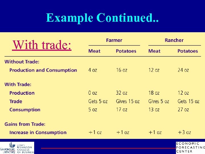
Example Continued. . With trade:

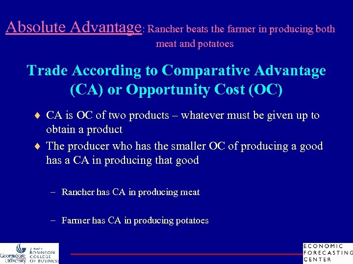
Absolute Advantage: Rancher beats the farmer in producing both meat and potatoes Trade According to Comparative Advantage (CA) or Opportunity Cost (OC) ¨ CA is OC of two products – whatever must be given up to obtain a product ¨ The producer who has the smaller OC of producing a good has a CA in producing that good – Rancher has CA in producing meat – Farmer has CA in producing potatoes

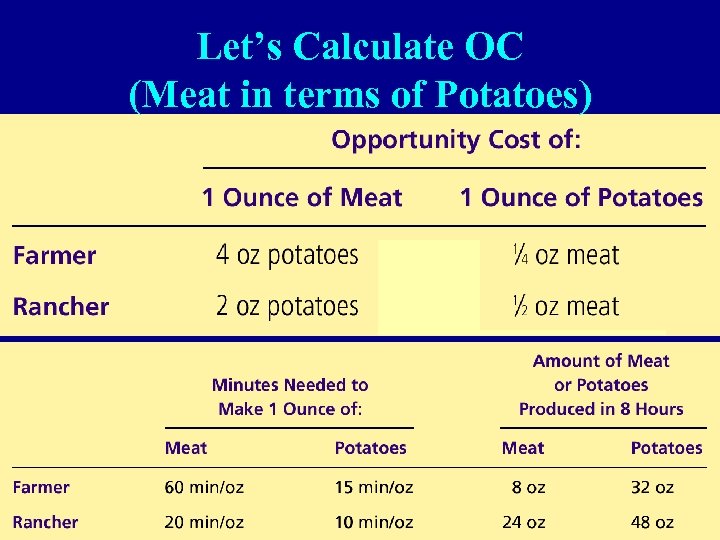
Let’s Calculate OC (Meat in terms of Potatoes)

Benefits of Trade ¨ Whenever potential trading parties have differences in opportunity costs, they can each benefit from trade. ¨ Trade can benefit everyone in a society because it allows people to specialize in activities in which they have a comparative advantage.

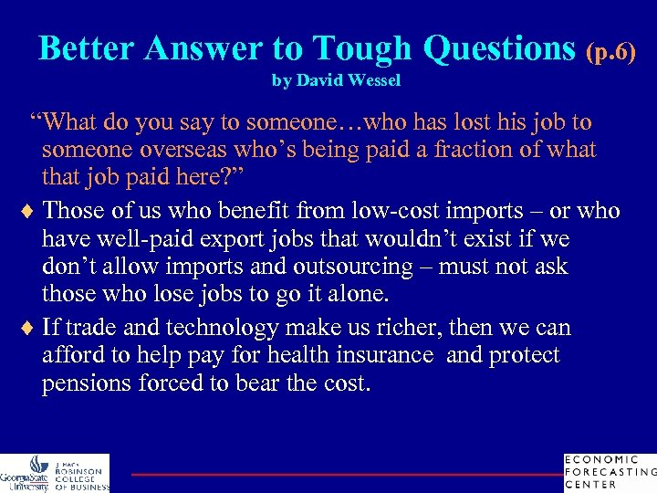
Better Answer to Tough Questions (p. 6) by David Wessel “What do you say to someone…who has lost his job to someone overseas who’s being paid a fraction of what that job paid here? ” ¨ Those of us who benefit from low-cost imports – or who have well-paid export jobs that wouldn’t exist if we don’t allow imports and outsourcing – must not ask those who lose jobs to go it alone. ¨ If trade and technology make us richer, then we can afford to help pay for health insurance and protect pensions forced to bear the cost.

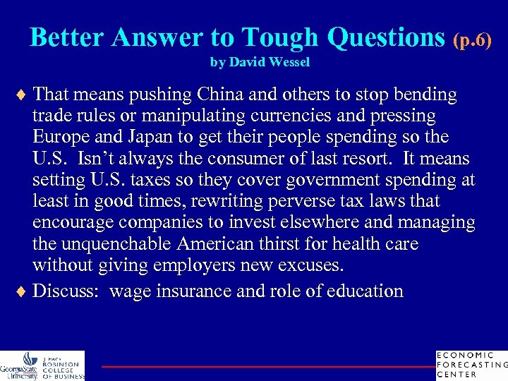
Better Answer to Tough Questions (p. 6) by David Wessel ¨ That means pushing China and others to stop bending trade rules or manipulating currencies and pressing Europe and Japan to get their people spending so the U. S. Isn’t always the consumer of last resort. It means setting U. S. taxes so they cover government spending at least in good times, rewriting perverse tax laws that encourage companies to invest elsewhere and managing the unquenchable American thirst for health care without giving employers new excuses. ¨ Discuss: wage insurance and role of education

Chapter 5 Elasticity

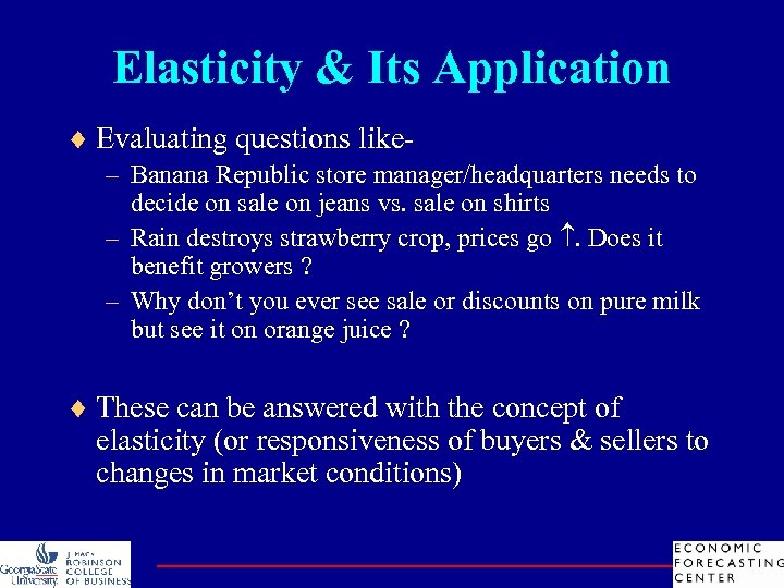
Elasticity & Its Application ¨ Evaluating questions like– Banana Republic store manager/headquarters needs to decide on sale on jeans vs. sale on shirts – Rain destroys strawberry crop, prices go . Does it benefit growers ? – Why don’t you ever see sale or discounts on pure milk but see it on orange juice ? ¨ These can be answered with the concept of elasticity (or responsiveness of buyers & sellers to changes in market conditions)

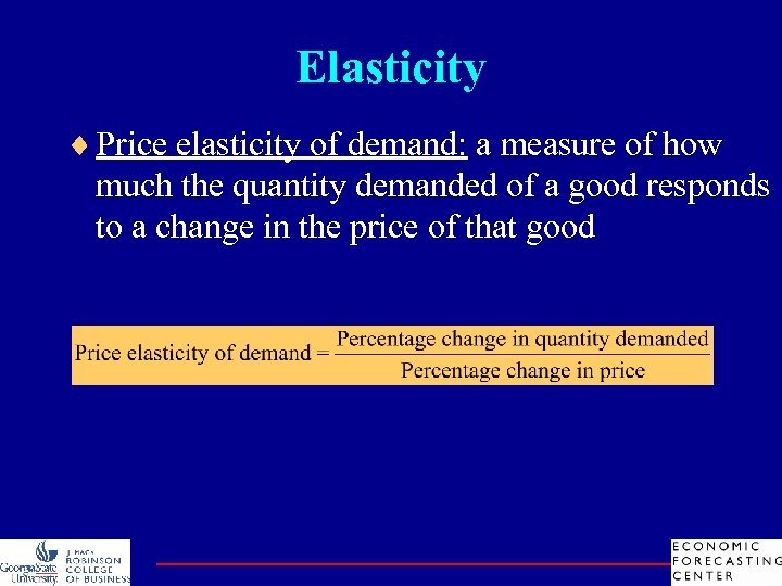
Elasticity ¨ Price elasticity of demand: a measure of how much the quantity demanded of a good responds to a change in the price of that good

Continued. . ¨ Two types of demand: – Elastic – responds a lot e. g. luxury cars ( luxuries) – Inelastic – not much change e. g. milk, certain food items, gasoline ( necessities) ¨ Preferences: Luxuries vs. Necessities ¨ Availability of close substitutes: Elastic – Butter & margarine; cars, booze ¨ Time horizon: – Gasoline – necessity in short run – Substitute long run (electric cars, walk, bike)

Elasticity ¨ Inelastic Demand – Quantity demanded does not respond strongly to price changes. – Price elasticity of demand is < one. ¨ Elastic Demand – Quantity demanded responds strongly to changes in price. – Price elasticity of demand is > one.

Demand Curves ¨ Question: Can I tell from the graphical shape of the demand curve what kind of elasticity the curve has? ¨ Answer: Yes, but not all the time.

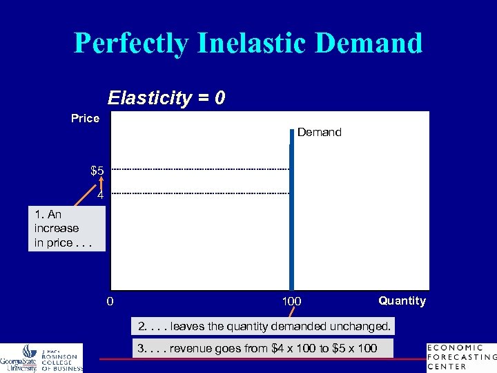
Perfectly Inelastic Demand Elasticity = 0 Price Demand $5 4 1. An increase in price. . . 0 100 Quantity 2. . leaves the quantity demanded unchanged. 3. . revenue goes from $4 x 100 to $5 x 100

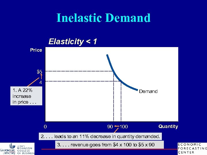
Inelastic Demand Elasticity < 1 Price $5 4 1. A 22% increase in price. . . Demand 0 90 100 Quantity 2. . leads to an 11% decrease in quantity demanded. 3. . revenue goes from $4 x 100 to $5 x 90

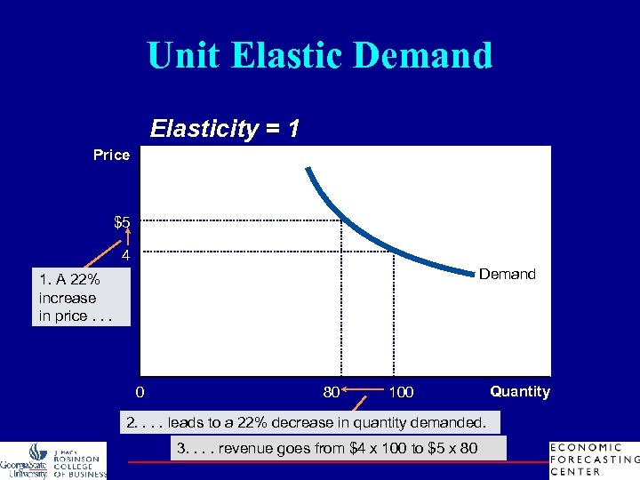
Unit Elastic Demand Elasticity = 1 Price $5 4 Demand 1. A 22% increase in price. . . 0 80 100 2. . leads to a 22% decrease in quantity demanded. 3. . revenue goes from $4 x 100 to $5 x 80 Quantity

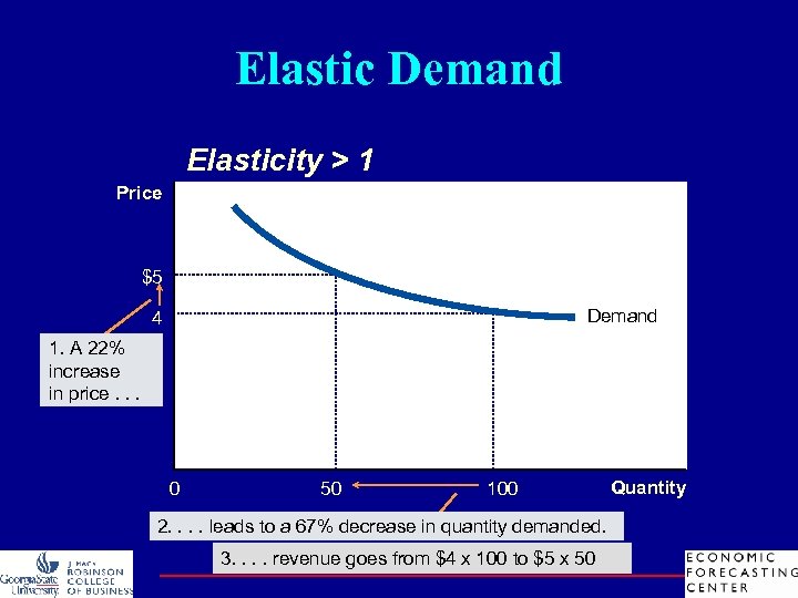
Elastic Demand Elasticity > 1 Price $5 Demand 4 1. A 22% increase in price. . . 0 50 100 2. . leads to a 67% decrease in quantity demanded. 3. . revenue goes from $4 x 100 to $5 x 50 Quantity

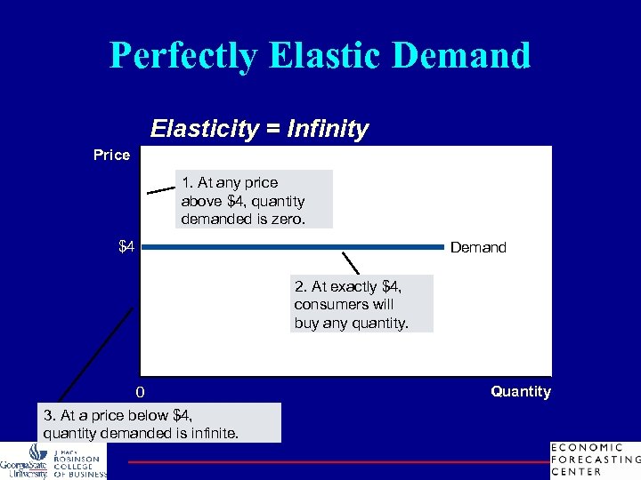
Perfectly Elastic Demand Elasticity = Infinity Price 1. At any price above $4, quantity demanded is zero. $4 Demand 2. At exactly $4, consumers will buy any quantity. 0 3. At a price below $4, quantity demanded is infinite. Quantity

Relationship Between Total Revenue (Sales) & Elasticity ¨ Total Revenue = Price x Qty Sold = P x Qty ¨ If demand is elastic, then a price decrease increases revenue ¨ If demand is inelastic, then a price increases revenue v. Example class to contribute

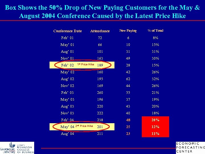
Box Shows the 50% Drop of New Paying Customers for the May & August 2004 Conference Caused by the Latest Price Hike Conference Date Attendance New Paying % of Total Feb’ 01 72 6 8% May’ 01 66 10 15% Aug’ 01 101 31 31% Nov’ 01 163 49 30% 189 28 15% May’ 02 160 42 26% Aug’ 02 195 62 32% Nov’ 02 169 44 26% Feb’ 03 260 55 21% May’ 03 196 37 19% Aug’ 03 220 43 20% Nov’ 03 222 40 18% Feb’ 04 238 48 20% 201 25 12% 211 23 11% Feb’ 02 May’ 04 Aug’ 04 1 st Price Hike 2 nd Price Hike

Applications of Supply, Demand & Elasticity ¨ Can good news for farmers be bad news for farmers? ¨ Wheat is inelastic: Bumper crop bad news

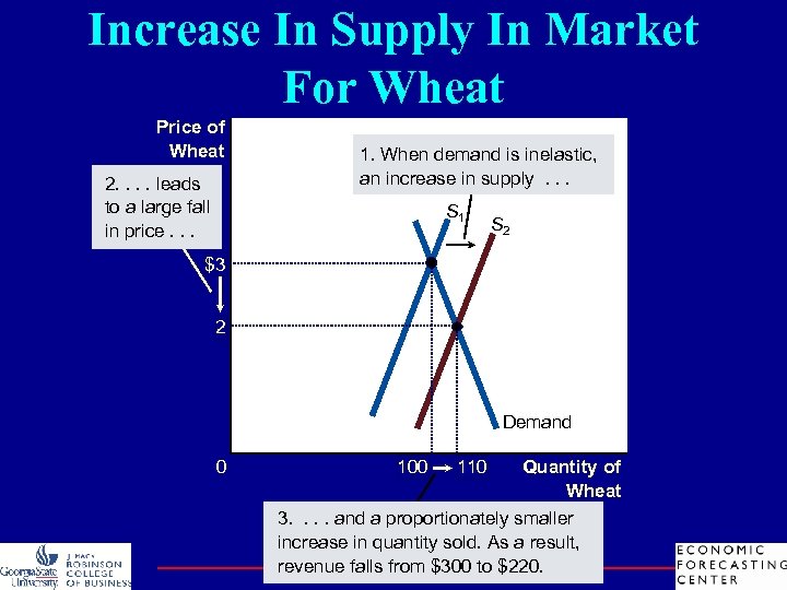
Increase In Supply In Market For Wheat Price of Wheat 2. . leads to a large fall in price. . . 1. When demand is inelastic, an increase in supply. . . S 1 S 2 $3 2 Demand 0 100 110 Quantity of Wheat 3. . and a proportionately smaller increase in quantity sold. As a result, revenue falls from $300 to $220.