Lecture 19 Nov 10 2010 Discrete event simulation

Lecture 19 Nov 10, 2010 Discrete event simulation (Ross) • discrete and continuous distributions • computationally generating random variable following various distributions. • repair problem

Exercise 2: (coupon collector’s problem) When you buy a can of soda, it contains a coupon with a label in 1: n. The labels on the can are random in the sense that, at any point during simulation, the probability that the next can you buy will contain label j is 1/n. The goal is the determine the average number of cans you need to buy before you have collected all the n coupons. Idea: create an array A of size n, all set to 0. Create another array to keep track of the number of cans to buy before all n coupons are collected. The size of this array B is m = the number of trials. Repeat generating a random number j in 1: n, and increment A(j) until all A(j) are > 0. At this point, set B(k) to sum(A) and repeat fro k = 1, 2, …, m.

Probability distributions • In a Discrete Event Simulation, you need to decide what probability distribution functions best model the events. in most situations, uniform distribution does not work. • Pseudorandom number generators generate numbers in a uniform distribution • One basic trick is to transform that uniform distribution into other distributions. • Some standard probability distributions are convenient to represent mathematically. • They may or may not represent reality, but can be useful simplification.

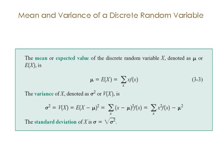Mean and Variance of a Discrete Random Variable

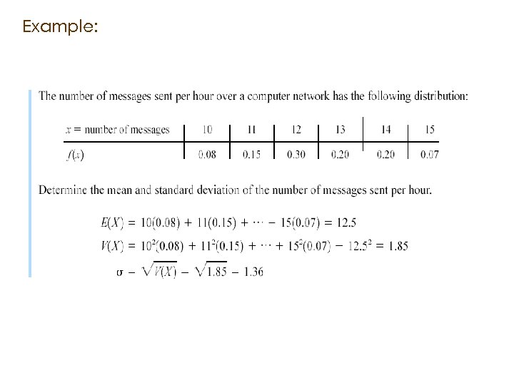Example:

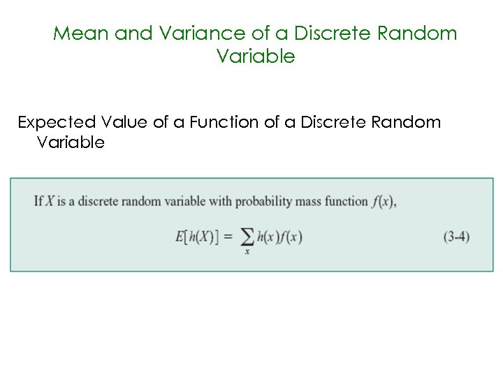Mean and Variance of a Discrete Random Variable Expected Value of a Function of a Discrete Random Variable

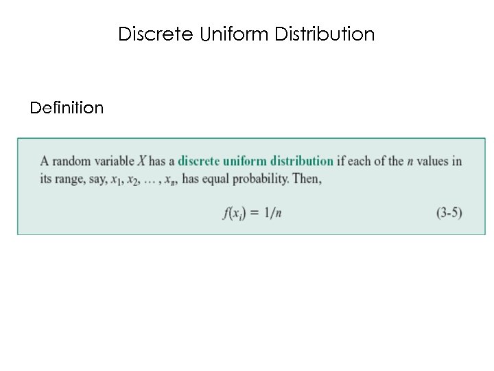Discrete Uniform Distribution Definition

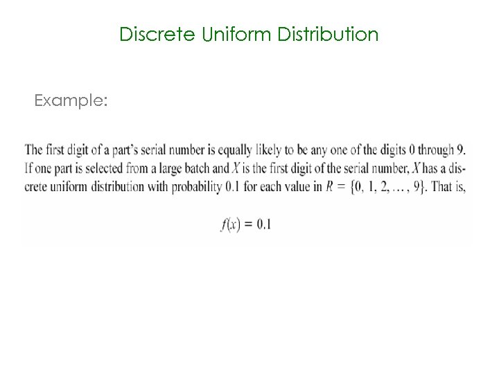Discrete Uniform Distribution Example:

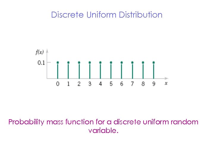Discrete Uniform Distribution Probability mass function for a discrete uniform random variable.

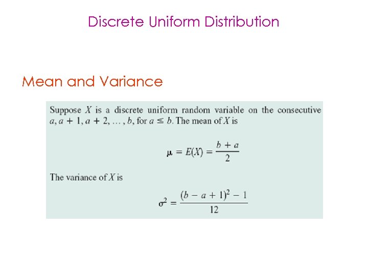Discrete Uniform Distribution Mean and Variance

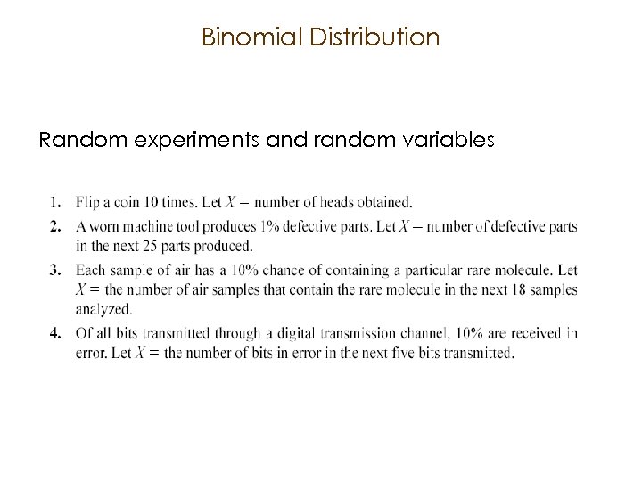Binomial Distribution Random experiments and random variables

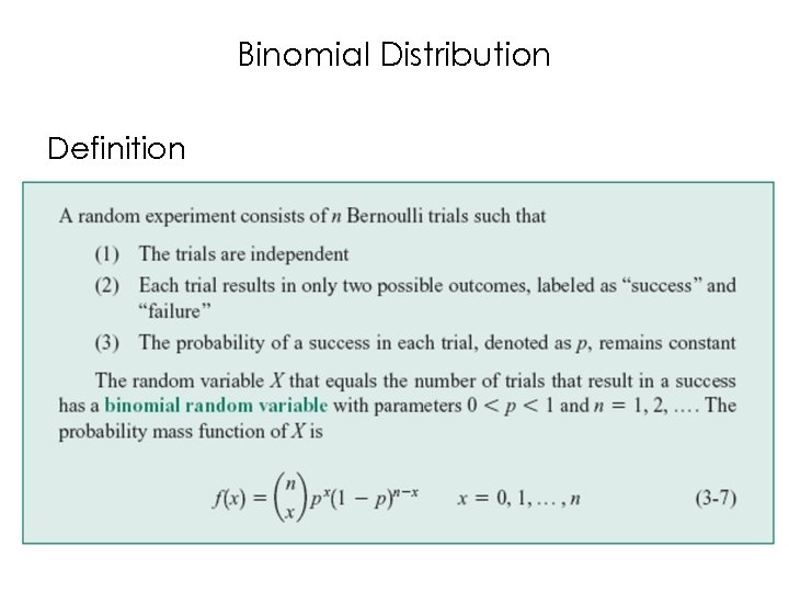Binomial Distribution Definition

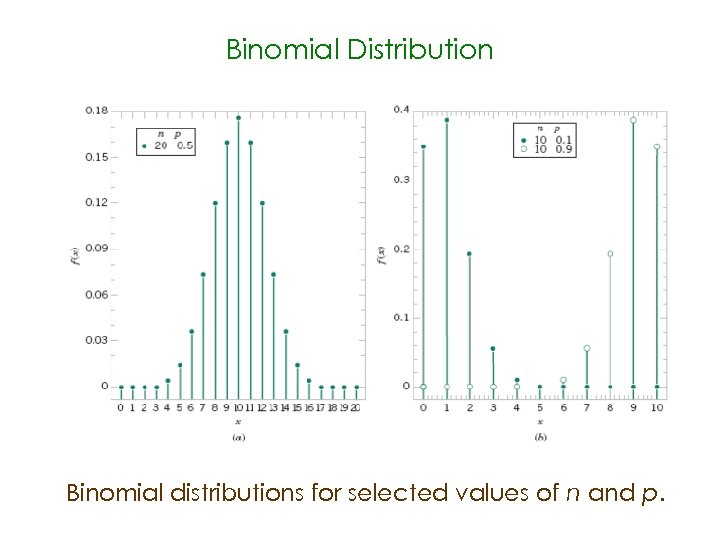Binomial Distribution Binomial distributions for selected values of n and p.

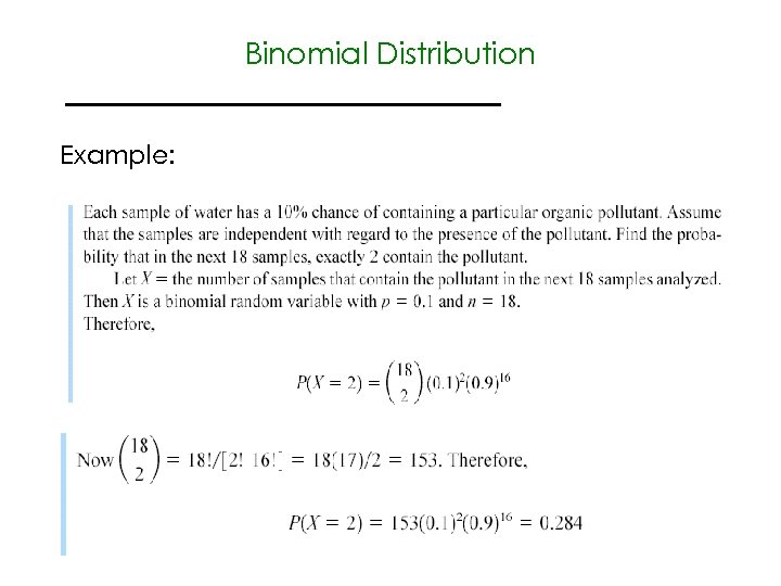Binomial Distribution Example:

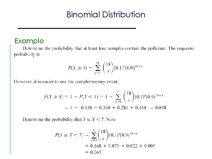Binomial Distribution Example

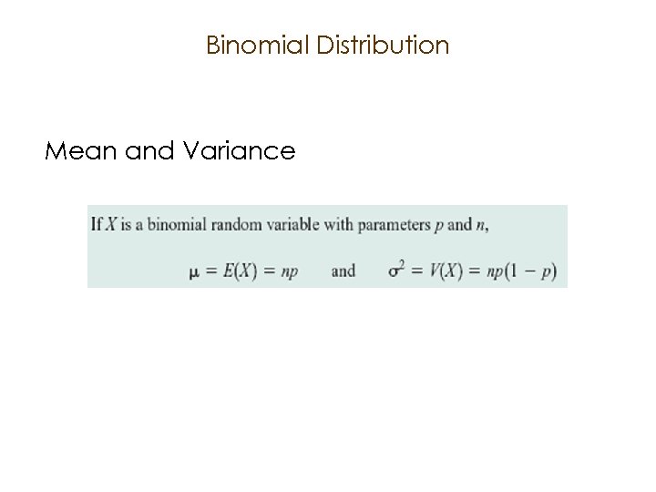Binomial Distribution Mean and Variance

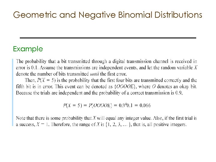Geometric and Negative Binomial Distributions Example

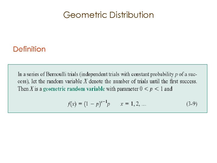Geometric Distribution Definition

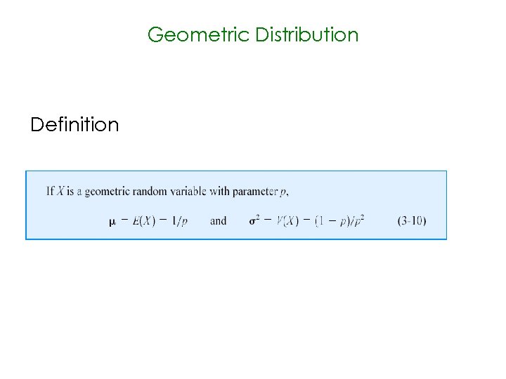Geometric Distribution Definition

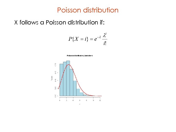Poisson distribution X follows a Poisson distribution if:

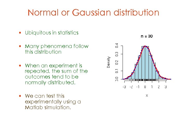Normal or Gaussian distribution § Ubiquitous in statistics § Many phenomena follow this distribution § When an experiment is repeated, the sum of the outcomes tend to be normally distributed. § We can test this experimentally using a Matlab simulation.

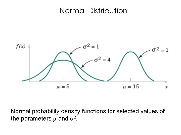Normal Distribution Normal probability density functions for selected values of the parameters and 2.

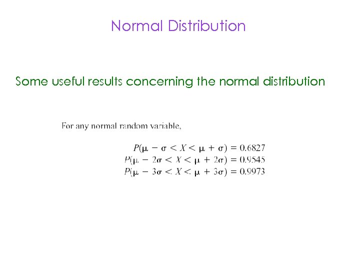Normal Distribution Some useful results concerning the normal distribution

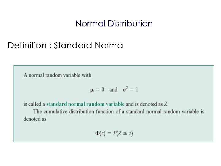Normal Distribution Definition : Standard Normal

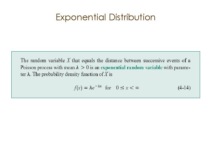Exponential Distribution

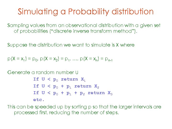Simulating a Probability distribution Sampling values from an observational distribution with a given set of probabilities (“discrete inverse transform method”). Suppose the distribution we want to simulate is X where p(X = x 1) = p 0, p(X = x 2) = p 1, …, p(X = xn) = pn-1 Generate a random number U If U < p 0 return X 1 If U < p 0 + p 1 return X 2 If U < p 0 + p 1 + p 2 return X 3 etc. This can be speeded up by sorting p so that the larger intervals are processed first, reducing the number of steps.

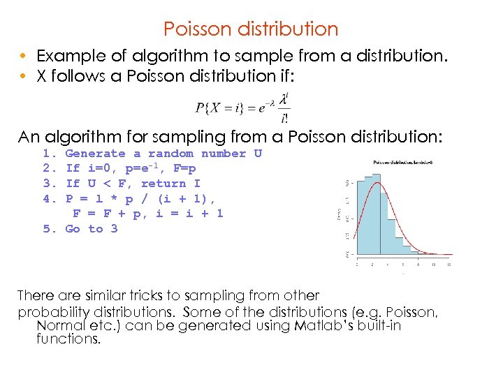Poisson distribution • Example of algorithm to sample from a distribution. • X follows a Poisson distribution if: An algorithm for sampling from a Poisson distribution: 1. 2. 3. 4. Generate a random number U If i=0, p=e-l, F=p If U < F, return I P = l * p / (i + 1), F = F + p, i = i + 1 5. Go to 3 There are similar tricks to sampling from other probability distributions. Some of the distributions (e. g. Poisson, Normal etc. ) can be generated using Matlab’s built-in functions.

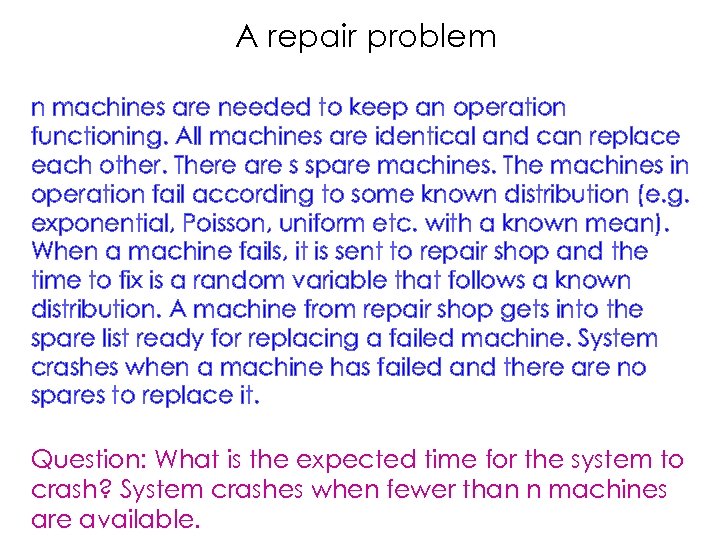A repair problem n machines are needed to keep an operation functioning. All machines are identical and can replace each other. There are s spare machines. The machines in operation fail according to some known distribution (e. g. exponential, Poisson, uniform etc. with a known mean). When a machine fails, it is sent to repair shop and the time to fix is a random variable that follows a known distribution. A machine from repair shop gets into the spare list ready for replacing a failed machine. System crashes when a machine has failed and there are no spares to replace it. Question: What is the expected time for the system to crash? System crashes when fewer than n machines are available.

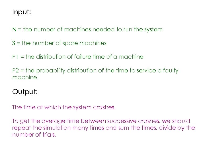Input: N = the number of machines needed to run the system S = the number of spare machines P 1 = the distribution of failure time of a machine P 2 = the probability distribution of the time to service a faulty machine Output: The time at which the system crashes. To get the average time between successive crashes, we should repeat the simulation many times and sum the times, divide by the number of trials.

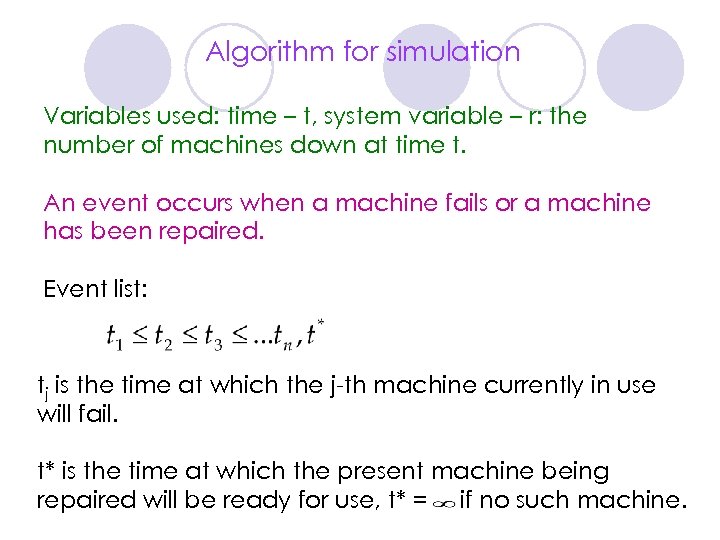Algorithm for simulation Variables used: time – t, system variable – r: the number of machines down at time t. An event occurs when a machine fails or a machine has been repaired. Event list: tj is the time at which the j-th machine currently in use will fail. t* is the time at which the present machine being repaired will be ready for use, t* = if no such machine.

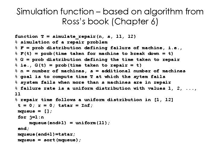Simulation function – based on algorithm from Ross’s book (Chapter 6) function T = simulate_repair(n, s, l 1, l 2) % simulation of a repair problem % F = prob distribution defining failure of machine, i. e. , % F(t) = prob(time taken for machine to break down = t) % G = prob distribution defining the time taken to repair % ie. , G(t) = prob(time taken to repair = t) % n = number of machines, s = additional number of machines % goal is to compute time T at which the sytem fails % system fails when more than s machines are in repair % failure rate is a uniform distribution with values 1, 2, . . . , l 1 % repair time follows a uniform distribution in [1, l 2] t = 0; r = 0; tstar = Inf; mqueue = []; for j=1: n mqueue(end+1) = uniform(l 1); end; mqueue(end+1)=tstar; mqueue = sort(mqueue);

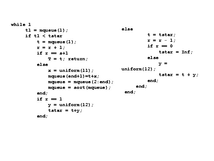while 1 t 1 = mqueue(1); if t 1 < tstar t = mqueue(1); r = r + 1; if r == s+1 T = t; return; else x = uniform(l 1); mqueue(end+1)=t+x; mqueue = mqueue(2: end); mqueue = sort(mqueue); end; if r == 1 y = uniform(l 2); tstar = t+y; end; else t = tstar; r = r - 1; if r == 0 tstar = Inf; else y = uniform(l 2); tstar = t + y; end;

It is easy to modify the code so that the distributions (for failure time and repair time) are not uniform, but say Poisson, exponential or normal etc. Exercise: Try replacing uniform by Poisson or exponential and compute the expected time for crash. Does it increase the expected time before the system crashes (given the same mean)?

Service queue simulation Problem: Each customer joins a queue serviced by a single server. The arrival time of the customer is a random number given by a known distribution. Time to service obeys a known (possibly different) probability distribution. Assume that there a total of N customers. (N is known. ) Goal is to calculate the average time a customer has to wait in the service line? We may also want to calculate the average waiting time of the k-th customer. Variations: 1) assume that after some time T, no additional customer allowed. 2) There are two service providers.

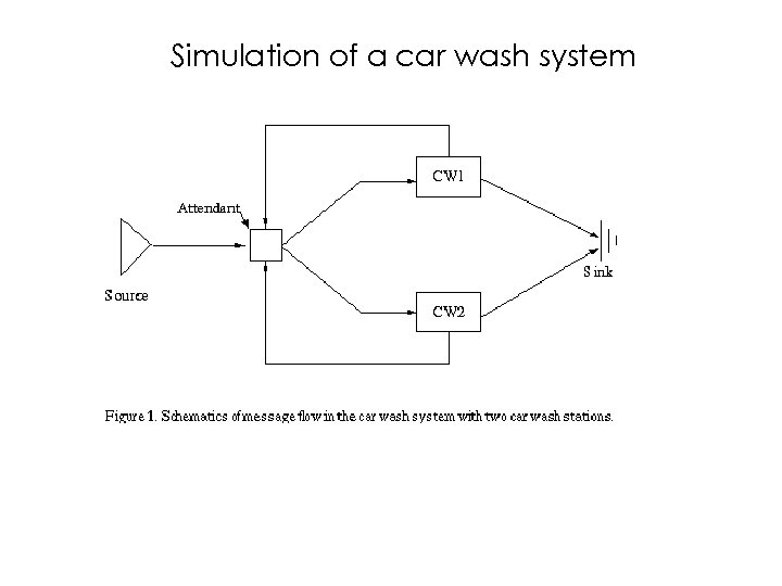Simulation of a car wash system