6d8f267e41c83dbe41633af688ef2f7d.ppt
- Количество слайдов: 14
 Lecture 18: Thurs. , March 18
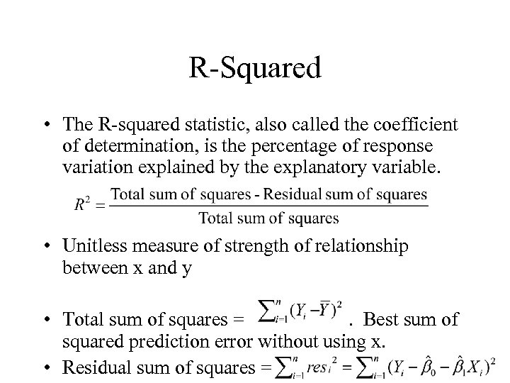 R-Squared • The R-squared statistic, also called the coefficient of determination, is the percentage of response variation explained by the explanatory variable. • Unitless measure of strength of relationship between x and y • Total sum of squares =. Best sum of squared prediction error without using x. • Residual sum of squares =
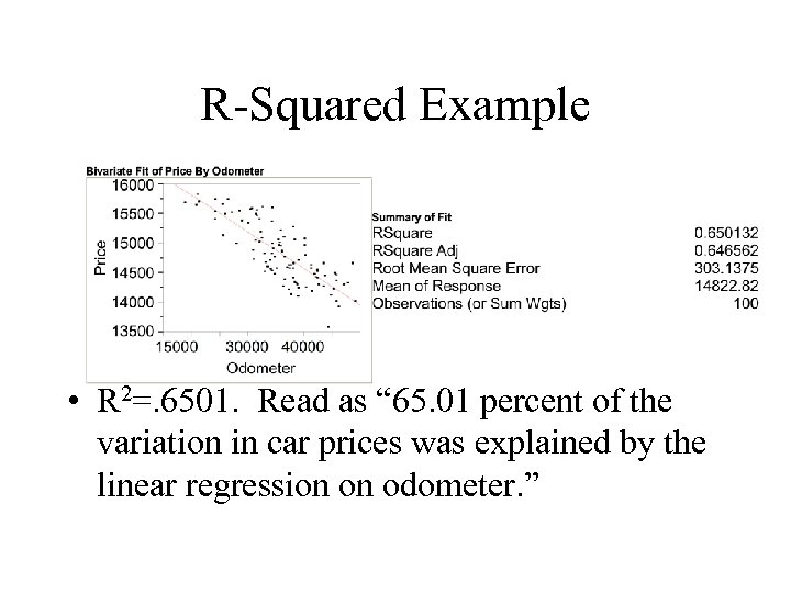 R-Squared Example • R 2=. 6501. Read as “ 65. 01 percent of the variation in car prices was explained by the linear regression on odometer. ”
 Interpreting 2 R • R 2 takes on values between 0 and 1, with higher R 2 indicating a stronger linear association. • For simple linear regression, R 2 is the square of the correlation between the predictor and the response. • If the residuals are all zero (a perfect fit), then R 2 is 1. If the least squares line has slope 0, R 2 will be 0. • R 2 is useful as a unitless summary of the strength of linear association.
 Caveats about 2 R – R 2 is not useful for assessing model adequacy, i. e. , does simple linear regression model hold (use residual plots) or whether or not there is an association (use test of vs. ) – A good R 2 depends on the context. In precise laboratory work, R 2 values under 90% might be too low, but in social science contexts, when a single variable rarely explains great deal of variation in response, R 2 values of 50% may be considered remarkably good.
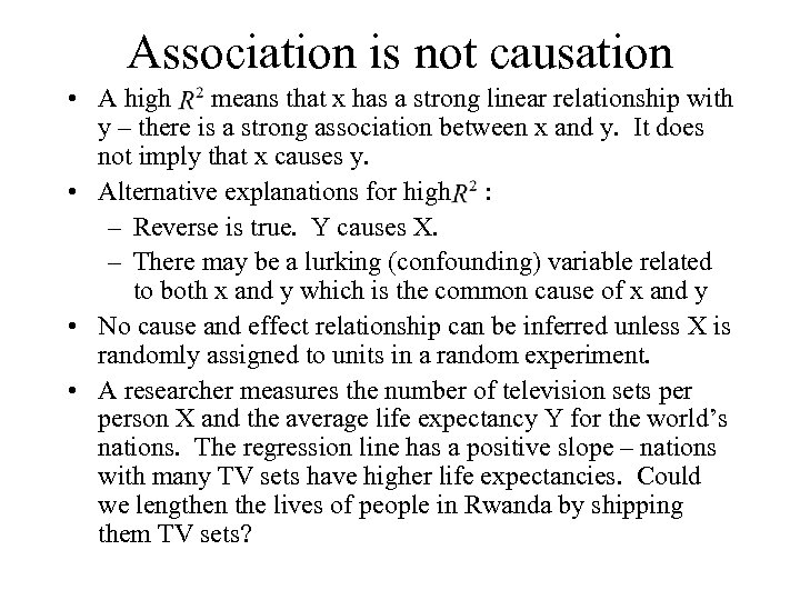 Association is not causation • A high means that x has a strong linear relationship with y – there is a strong association between x and y. It does not imply that x causes y. • Alternative explanations for high : – Reverse is true. Y causes X. – There may be a lurking (confounding) variable related to both x and y which is the common cause of x and y • No cause and effect relationship can be inferred unless X is randomly assigned to units in a random experiment. • A researcher measures the number of television sets person X and the average life expectancy Y for the world’s nations. The regression line has a positive slope – nations with many TV sets have higher life expectancies. Could we lengthen the lives of people in Rwanda by shipping them TV sets?
 House Prices and Crime • A community in the Philadelphia area is interested in how crime rates affect property values. If low crime rates increase property values, the community may be able to cover the costs of increased police protection by gains in tax revenues from higher property values. Data on the average housing price and crime rate (per 1000 population) for communities in Pennsylvania near Philadelphia for 1996 are shown in housecrime. JMP.
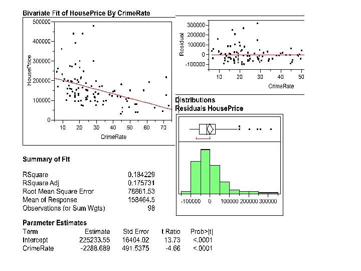
 Questions 1. Can you deduce a cause-and-effect relationship from these data? What are other explanations for the association between housing prices and crime rate other than that high crime rates cause low housing prices? 2. Does the ideal simple linear regression model appear to hold?
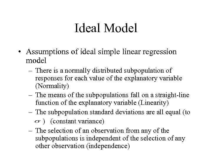 Ideal Model • Assumptions of ideal simple linear regression model – There is a normally distributed subpopulation of responses for each value of the explanatory variable (Normality) – The means of the subpopulations fall on a straight-line function of the explanatory variable (Linearity) – The subpopulation standard deviations are all equal (to ) (constant variance) – The selection of an observation from any of the subpopulations is independent of the selection of any other observation (independence)
 Regression Diagnostics • The conditions required for inference from simple linear regression must be checked: – Linearity. Diagnostic: Residual plot – Constant variance. Diagnostic: Residual plot. – Normality. Diagnostic: Histogram of residuals/Normal probability plot of residuals. – Independence. Diagnostic: Residual plot. – Outliers and influential points. Diagnostic: Scatterplot, Cook’s Distances.
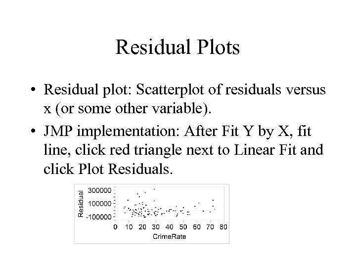 Residual Plots • Residual plot: Scatterplot of residuals versus x (or some other variable). • JMP implementation: After Fit Y by X, fit line, click red triangle next to Linear Fit and click Plot Residuals.
 Use of Residual Plot • Use residual plot to look for nonlinearity and nonconstant variance • If the ideal simple linear regression model holds, the residual plot should look like random scatter – there should be no pattern in the residual plot – A pattern in the mean of the residuals, i. e. , the residuals have a mean less than zero for some range of x and greater than zero for another range of x indicates nonlinearity. – A pattern in the variance of the residuals, i. e. , the residuals have a greater variance for some range of x and less variance for another range of x indicates nonconstant variance. • Look for marked patterns. No residual plot looks perfectly like random scatter.
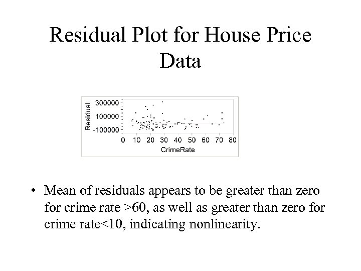 Residual Plot for House Price Data • Mean of residuals appears to be greater than zero for crime rate >60, as well as greater than zero for crime rate<10, indicating nonlinearity.


