Lecture 17 Interaction Plots Simple Linear

Lecture 17 • Interaction Plots • Simple Linear Regression (Chapter 18. 118. 2) • Homework 4 due Friday. JMP instructions for question 15. 41 are actually for question 15. 35.

18. 1 Introduction • In Chapters 18 to 20 we examine the relationship between interval variables via a mathematical equation. • The motivation for using the technique: – Forecast the value of a dependent variable (y) from the value of independent variables (x 1, x 2, …xk. ). – Analyze the specific relationships between the independent variables and the dependent variable.

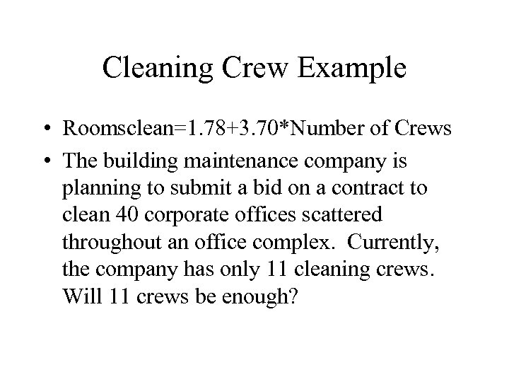
Uses of Regression Analysis • A building manager company plans to submit a bid on a contract to clean 40 corporate offices scattered throughout an office complex. The costs incurred by the company are proportional to the number of cleaning crews needed for this task. How many crews will be enough? • The product manager in charge of a brand of children’s cereal would like to predict demand during the next year. She has available the following “predictor” variables: price of the product, number of children in target market, price of competitors’ products, effectiveness of advertising, annual sales this year and previous year

Uses of Regression Analysis • A community in the Philadelphia area is interested in how crime rates affect property values. If low crime rates increase property values, the community might be able to cover the cost of increased police protection by gains in tax revenues from higher property values. • A real estate agent wants to more accurately predict the selling price of houses. She believes the following variables affect the price of a house: Size of house (sq. feet), number of bedrooms, frontage of lot, condition and location.

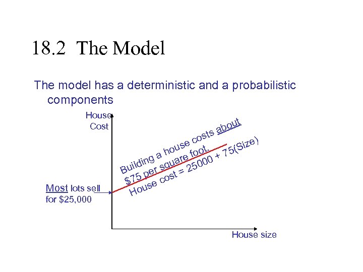18. 2 The Model The model has a deterministic and a probabilistic components House Cost Most lots sell for $25, 000 out ab s ost c ize) se t. (S ou a h re foo 0 + 75 g ldin r squa 2500 Bui pe t= 75 e cos $ ous H House size

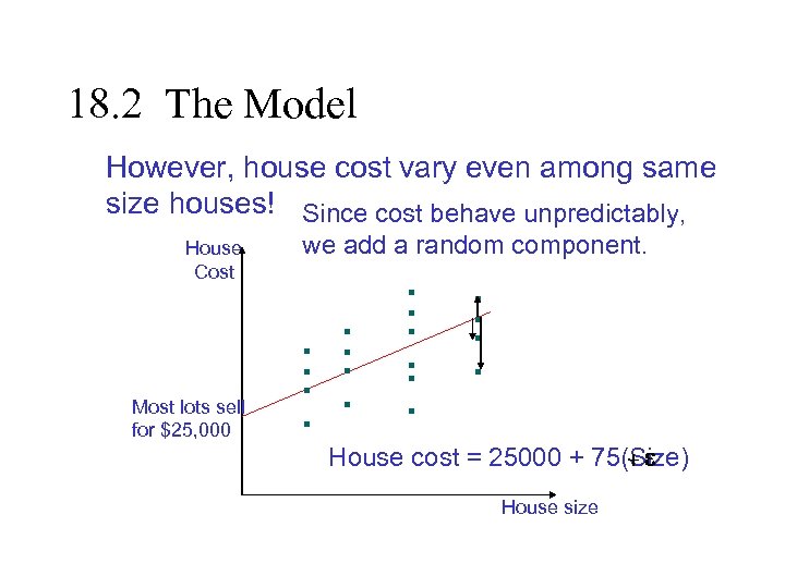18. 2 The Model However, house cost vary even among same size houses! Since cost behave unpredictably, House Cost Most lots sell for $25, 000 we add a random component. +e House cost = 25000 + 75(Size) House size

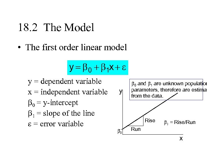18. 2 The Model • The first order linear model y = dependent variable x = independent variable b 0 = y-intercept b 1 = slope of the line e = error variable y b 0 and b 1 are unknown population parameters, therefore are estimat from the data. Rise b 0 b 1 = Rise/Run x

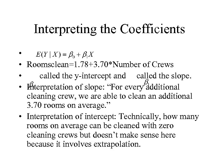Interpreting the Coefficients • • Roomsclean=1. 78+3. 70*Number of Crews • called the y-intercept and called the slope. • Interpretation of slope: “For every additional cleaning crew, we are able to clean an additional 3. 70 rooms on average. ” • Interpretation of intercept: Technically, how many rooms on average can be cleaned with zero cleaning crews but doesn’t make sense here because it involves extrapolation.

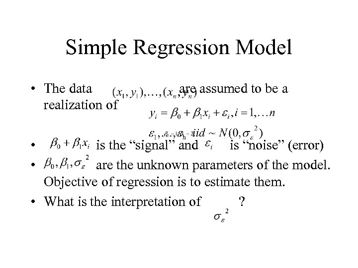Simple Regression Model • The data realization of • • are assumed to be a is the “signal” and is “noise” (error) are the unknown parameters of the model. Objective of regression is to estimate them. • What is the interpretation of ?

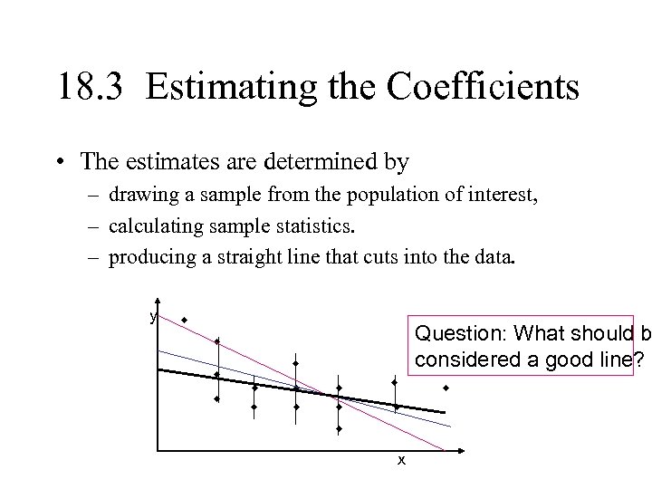18. 3 Estimating the Coefficients • The estimates are determined by – drawing a sample from the population of interest, – calculating sample statistics. – producing a straight line that cuts into the data. y w Question: What should b considered a good line? w w w w x w

The Least Squares (Regression) Line A good line is one that minimizes the sum of squared differences between the points and the line.

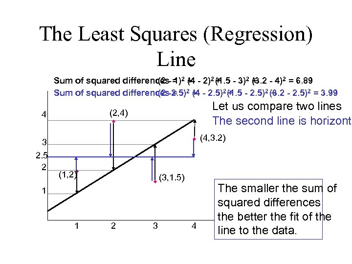The Least Squares (Regression) Line Sum of squared differences- = 2 + - 2)2 (1. 5 - 3)2 + - 4)2 = 6. 89 (2 1) (4 + (3. 2 Sum of squared differences-2. 5)2 + - 2. 5)2 (1. 5 - 2. 5)2 (3. 2 - 2. 5)2 = 3. 99 (2 = (4 + + 3 2. 5 2 Let us compare two lines The second line is horizonta (2, 4) w 4 w (4, 3. 2) w (1, 2) w (3, 1. 5) 1 1 2 3 4 The smaller the sum of squared differences the better the fit of the line to the data.

The Estimated Coefficients To calculate the estimates of the line coefficients, that minimize the differences between the data points and the line, use the formulas: The regression equation that estimate the equation of the first order linear m is:

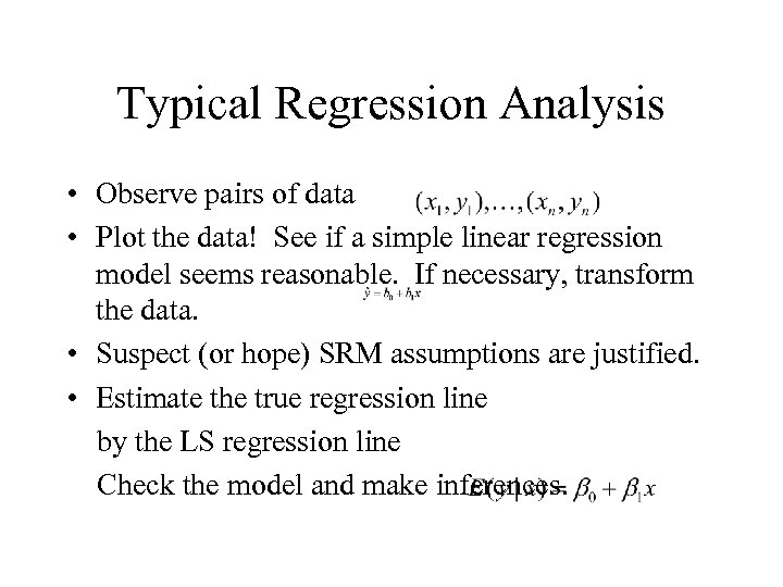Typical Regression Analysis • Observe pairs of data • Plot the data! See if a simple linear regression model seems reasonable. If necessary, transform the data. • Suspect (or hope) SRM assumptions are justified. • Estimate the true regression line by the LS regression line Check the model and make inferences.

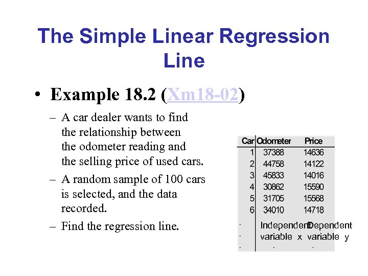The Simple Linear Regression Line • Example 18. 2 (Xm 18 -02) – A car dealer wants to find the relationship between the odometer reading and the selling price of used cars. – A random sample of 100 cars is selected, and the data recorded. – Find the regression line. Independent Dependent variable x variable y

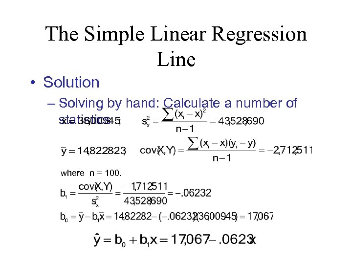The Simple Linear Regression Line • Solution – Solving by hand: Calculate a number of statistics where n = 100.

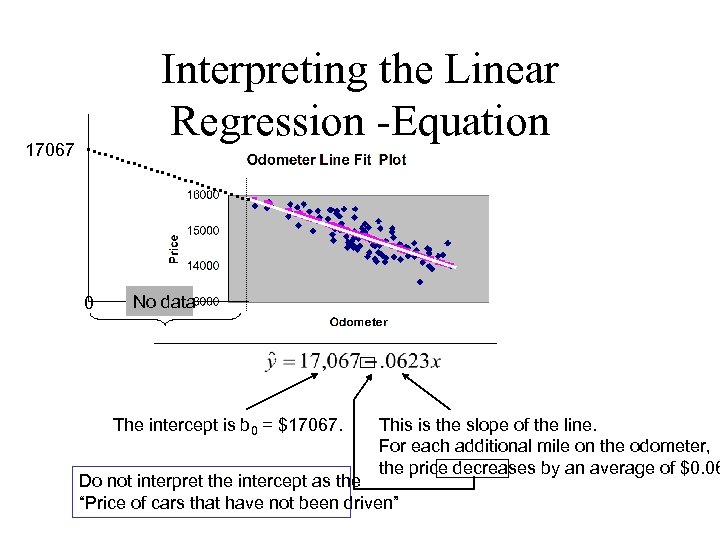Interpreting the Linear Regression -Equation 17067 0 No data The intercept is b 0 = $17067. This is the slope of the line. For each additional mile on the odometer, the price decreases by an average of $0. 06 Do not interpret the intercept as the “Price of cars that have not been driven”

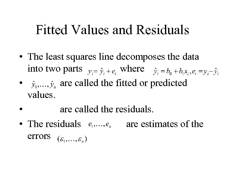Fitted Values and Residuals • The least squares line decomposes the data into two parts where • are called the fitted or predicted values. • are called the residuals. • The residuals are estimates of the errors

18. 4 Error Variable: Required Conditions • The error e is a critical part of the regression model. • Four requirements involving the distribution of e must be satisfied. – – The probability distribution of e is normal. The mean of e is zero: E(e) = 0. The standard deviation of e is se for all values of x. The set of errors associated with different values of y are all independent.

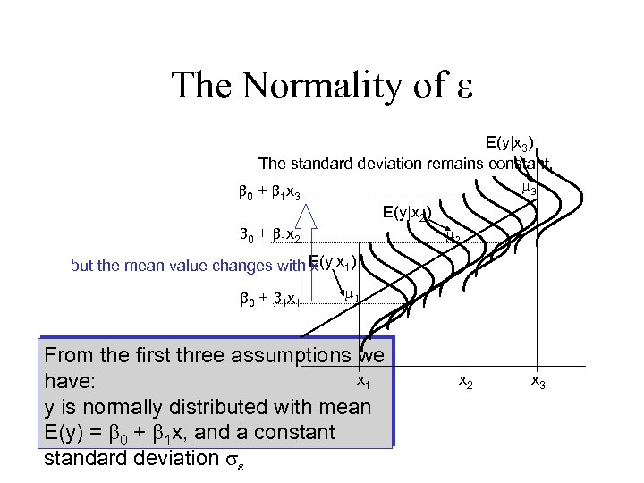The Normality of e E(y|x 3) The standard deviation remains constant, m 3 b 0 + b 1 x 3 E(y|x 2) b 0 + b 1 x 2 m 2 but the mean value changes with E(y|x 1) x b 0 + b 1 x 1 m 1 From the first three assumptions we x 1 have: y is normally distributed with mean E(y) = b 0 + b 1 x, and a constant standard deviation se x 2 x 3

Estimating • The standard error of estimate (root mean squared error) is an estimate of • The standard error of estimate is basically the standard deviation of the residuals. • If the simple regression model holds, then approximately – 68% of the data will lie within one – 95% of the data will lie within two of the LS line.

Cleaning Crew Example • Roomsclean=1. 78+3. 70*Number of Crews • The building maintenance company is planning to submit a bid on a contract to clean 40 corporate offices scattered throughout an office complex. Currently, the company has only 11 cleaning crews. Will 11 crews be enough?

Practice Problems • 18. 4, 18. 10, 18. 12