Lecture 13 Introduction to Keynesian Macroeconomics The

Lecture 13 Introduction to Keynesian Macroeconomics • The Birth of Macro in the Great Depression • Elements of National Income Accounting • National Income Determination

Macro- and Microeconomics • Microeconomics – Microeconomics is the study of how individual households and firms make decisions and how they interact with one another in markets. • Macroeconomics – Macroeconomics is the study of the economy as a whole. – Its goal is to explain the economic changes that affect many households, firms, and markets at once. • Are Micro and Macro compatible? – Do they tell stories that jibe with one another? – Depends on whose story you believe.

The Birth of Macroeconomics in the Great Depression • Between 1929 and 1932, real output outside agriculture (as measured by private non-farm product) fell by 30 percent, non-farm employment by 22 percent, prices (wholesale industrial prices) by 22 percent, and money wages (hourly wage rates in manufacturing) by 16 percent. • The agricultural sector, which accounted for 23 percent of total employment in 1929 and 27 percent in 1932, as well as 10 and 14 percent of GDP, fared very differently. Real agricultural output remained constant, as did employment, but prices farmers received fell by 55 percent, while prices farmers paid in production fell by 33 percent and wage rates fell by 28 percent.

What Did Economists Make of This? • Myron W Watkins, “The Literature of the Crisis, ” Quarterly Journal of Economics, 47: 504 -532 (May, 1933) summarizes the conventional wisdom. • See Handout

Mandeville and Smith • Recall the difference mentioned between Mandeville and Smith with respect to how the economy works: For Mandeville, but not Smith luxury, fashion, etc are necessary for the economy to thrive. • What is the basis of this difference • See Handout 2.

J M Keynes and the Central Idea of Macro • Aggregate Demand Matters • See Handout 4.

National Income Accounting • Gross Domestic Product as the value of total output (production) – – – GDP (Y) is the sum of the following: Consumption (C) Investment (I) Government Purchases (G) Net Exports (NX = X - M) • Y = C + I + G + NX – Why are imports subtracted from exports in the calculation of GDP?

Investment in macroeconomics (and in NIA) and investment in ordinary language • In macroeconomics, investment is the commitment of output to specific physical forms of capital goods, the commitment of the command over resources represented by abstract purchasing power to plant, equipment, highways and other transportation infrastructure, houses, etc. • In ordinary language investment refers to the purchase of securities like stocks, bonds, CD’s (that’s certificates of deposit, not compact disks), the purchase of real estate for rental purposes, etc. • What’s the difference?

National Income Accounting (2) • Gross Domestic Product as the value of total income. – – GDP (Y) is the sum of the following: Consumption (C) Saving (S) Taxes (T) • Y=C+S+T

Saving in macroeconomics (and NIA) and saving in ordinary language • From an income perspective, saving in macroeconomics means income not spent on consumption goods and services • Saving (or rather savings) in ordinary language means accumulated wealth, including some physical capital, but also investment in the ordinary language sense of stocks, bonds, etc and even money in the bank in checking, savings, moneymarket accounts, and money kept under the mattress. • What’s the difference?

An Important National Income Identity • Suppose taxes and government spending are equal, so that G = T and net exports (NX) = 0. • Then Y = C + I + G + NX = C + S + T • So I = S – Does this result validate Smith, Watkins, and the latterday Smithians? • I = S is an accounting identity after the fact (ex post) because investment and saving are two ways of looking at the same thing: income which is not spent on consumption must be the same as output committed to specific capital goods. (This abstracts from government spending and taxes. )

An Important National Income Identity, cont’d • I = S is an accounting identity after the fact (ex post) because investment and saving are two ways of looking at the same thing: income which is not spent on consumption. • I = S is another way of saying that realized (ex post) output and income are identical.

And Before the Fact (Ex ante)? • Desired (ex ante) consumption need not equal realized (ex post) consumption, and neither desired (ex ante) investment nor desired (ex ante) saving need equal realized (ex post) levels. Nor need desired investment equal desired saving.

Another Concept: Expenditure • Expenditure is shorthand for “expenditure on goods and services. ” – Is saving expenditure? • Like other variables, expenditure can be distinguished between desired (ex ante) and realized (ex post) – Why might the two be different? • Desired expenditure is the sum of desired consumption and desired investment.

Desired, Undesired, and Realized Levels of GDP and Its Components • Some notation: we will use the subscript D to stand for “desired. ” And we will use the subscript U to stand for “undesired. ” The absence of a subscript will indicate realized levels. • By definition, realized levels are the sum of desired and undesired levels. For example, S = SD + SU I = ID + IU • Can you think of examples of undesired saving and investment?

The Statics and Dynamics of Income and Output • When desired levels of C, I, and S are equal to realized levels (ex ante = ex post), there is no in-built dynamic for output and income to change. Another way of saying this is that when desired expenditure is equal to income and output, there is no reason for income and output to change, at least not from the demand side. • When desired and realized levels of C, I, and S differ, there is an in-built dynamic for change—unless of course the departures of desired from realized levels offset one another.

An Example of Income Dynamics • Suppose NX = G = T = 0, C = 300, I = 100. So Y = C + I = 400. • What is S? • Suppose further that desired and realized levels of all variables are equal, so CD = 300, ID = 100. And ED = CD + ID = 400. • What is SD? • All of a sudden, people decide to spend less on consumption. CD falls to 250. What happens to ED and Y? – How would Adam Smith answer this question? – John Maynard Keynes?

Another Example • Suppose again NX = G = T = 0, C = 300, I = 100. So Y = C + I = 400. • And again that desired and realized levels of all variables are equal, so CD = 300, ID = 100. ED = CD + ID = 400. • All of a sudden, people decide to invest 120 rather than 100. What happens to ED and Y? – How would Adam Smith answer this question? – John Maynard Keynes?

The Keynesian (pronounced Canezian) System – In many of our examples we will assume that desired consumption is determined by income but that desired investment is not. We say that desired investment is autonomous. – Desired saving is the difference between income and desired consumption

A Simple Model of Income Determination Expenditure (E) 500 400 ED = Y 300 100 CD = 0. 75 Y 200 CD + ID ID 45° line 100 200 300 400 500 Income (Y)

A Simple Model of Income Determination: What Happens When I Increases? Expenditure (E) 500 480 ED = Y 400 200 CD + I 300 CD + Δ ID 120 100 CD = 0. 75 Y ID 45° line 100 200 300 ID + Δ ID = 120 400 480 500 Income (Y)

J M Keynes and the Central Idea of Macro • Aggregate Demand Matters • Now we can answer the question: matters for what? – Determination of Demand for Output (Income) and Employment. – The Demand for Employment is determined by an Aggregate Production Function which relates output to employment.

Hungry Helen’s Production Function (Lecture 5) Quantity of Output (cookies per hour) Production function 150 140 130 120 110 100 90 80 70 60 50 40 30 20 10 0 1 2 3 4 5 Number of Workers Hired Copyright © 2004 South -Western

Lecture 14 November 7, 2005 • The multiplier • The role of money • Money creation and the money multiplier • The Central Bank and its functions

The Multiplier • Let ΔI = 20. What happens to Y? ΔY = 80. Why? First round of expenditure: ΔI = 20 Second round of expenditure: MPC x ΔI = 0. 75 x 20 = 15 Third round of expenditure: MPC x ΔI = MPC 2 x ΔI = 0. 75 x 20 = 0. 75 x 15 = 11. 25 Summing all rounds: ΔY = (1 + MPC 2 + MPC 3 + …) ΔI = 1/(1 – MPC) ΔI Or • ΔY / ΔI = 1/(1 – MPC) = 1/(1 – 0. 75) = 1/ 0. 25 = 4.

Convergence of the Multiplier Sum to 1/(1 – MPC) • Let X = (1 + MPC 2 + MPC 3 + …) • Then MPC x X = (MPC + MPC 2 + MPC 3 + …) • Subtract the 2 nd equation from the 1 st: X – MPC x X = 1 • Or X (1 – MPC) = 1 • Or X = 1/(1 – MPC) • Holds for MPC < 1

What Happens When Investment Demand Rises? Suppose E = ED, MPC = 0. 75 • Period 0: ID = 100, Y = 400, CD = 300, E = ED = CD + ID = 400, SD = Y – CD = 100, Y – E = IU = 0, I = ID + IU = SD + SU = 100 • Period 1: ID = 120, Y = 400, CD = 300, E = ED = CD + ID = 420, SD = Y – CD = 100, Y – E = IU = -20, I = ID + IU = SD + SU = 100 • Period 2: ID = 120, Y = 420, CD = 315, E = ED = CD + ID = 435, SD = Y – CD = 105, Y – E = IU = -15, I = ID + IU = SD + SU = 105 • Period 3: ID = 120, Y = 435, CD = 326. 25, E = ED = CD + ID = 446. 25, SD = Y – CD = 108. 75, Y – E = IU = - 11. 25, I = ID + IU = SD + SU = 108. 75

A Simple Model of Income Determination: What Happens When I Increases? Expenditure (E) 500 480 ED = Y 400 200 CD + I 300 CD + Δ ID 120 100 CD = 0. 75 Y ID 45° line 100 200 300 ID + Δ ID = 120 400 480 500 Income (Y)

Money Creation • How do businesspeople get money for investment when they wish to expand capacity, as in the previous example? • When the economy soured in 2001, the Federal Reserve lowered interest rates, and lots of folks refinanced mortgages to take advantage of the lower rates. • With lower interest rates, people could maintain the same monthly payment on the mortgage, with a higher debt. • Many did so, taking the difference between the new (higher) debt and the old debt in cash. • Or they could keep debt at the same level and lower their monthly payment. • In either case they had more cash to spend. • When they spent this money, they added to aggregate demand, in effect pushing the consumption function upward, and moving the equilibrium in the direction of greater output, income, and employment. • Where did the money come from for these new loans?

Money in the U. S. Economy (2001) Billions of Dollars M 2 $5, 455 • Savings deposits • Small time deposits • Money market mutual funds • A few minor categories ($4, 276 billion) $1, 179 0 M 1 • Demand deposits • Traveler’s checks • Other checkable deposits ($599 billion) • Currency ($580 billion) • Everything in M 1 ($1, 179 billion) Copyright© 2003 Southwestern/Thomson Learning

Money Creation with Fractional. Reserve Banking • This T-Account shows a bank that… – accepts deposits, First National Bank – keeps a portion Assets as reserves, – and lends out Reserves the rest. $10. 00 – It assumes a reserve ratio Loans $90. 00 of 10%. Total Assets $100. 00 Liabilities Deposits $100. 00 Total Liabilities $100. 00

Money Creation with Fractional. Reserve Banking (2) • This T-Account shows a second bank that… – accepts deposits, Second – keeps a portion Assets as reserves, – and lends out Reserves the rest. $9. 00 – It assumes a reserve ratio Loans of 10%. $81. 00 Total Assets $90. 00 National Bank Liabilities Deposits $90. 00 Total Liabilities $90. 00

Money Creation with Fractional. Reserve Banking (3) • And now a third bank that… – accepts deposits, Third National Bank – keeps a portion Assets as reserves, – and lends out Reserves the rest. $8. 10 – It assumes a reserve ratio Loans $72. 90 of 10%. Total Assets $81. 00 Liabilities Deposits $81. 00 Total Liabilities $81. 00

Money Creation with Fractional. Reserve Banking • When one bank loans money, that money is generally deposited into another bank. • This creates more deposits and more reserves to be lent out. • When a bank makes a loan from its reserves, the money supply increases.

The Money Multiplier • How much money does each bank create? First National Bank: $90 Second National Bank: $81 Third National Bank: $72. 90 … • How much money is eventually created by all the banks together? • The money multiplier is the amount of money the banking system generates with each dollar of reserves. • Let L = 1 – R, where R is the reserve ratio. Then – – First round lending on the basis of a $1 deposit is L Second round lending is L 2 Third round lending is L 3 Summing the initial deposit and all the lending, we have 1 + L + L 2 + L 3 + L 4 + … • Look familiar?

A Familiar Formula for the Money Multiplier • 1 + L 2 + L 3 + L 4 + … = 1/(1 – L) • But L = 1 – R, so 1/(1 – L) = 1/R, which is to say that the money multiplier is 1 divided by the reserve ratio. • For example, with a reserve ratio of 10%, the money multiplier is 10.

Central Banks • A central bank is a bank for banks • The US central bank is the Federal Reserve • Central banks perform two basic functions – Provide loans for banks when the banks face demands for cash which exceed their available reserves—lender of last resort – Control the money supply • Are these two roles compatible?

Tools of Monetary Control • Open Market Operations • Discount Rate (the rate the Fed charges banks on loans) • Reserve Requirements

Tools of Monetary Control • Open Market Operations • Discount Rate (the rate the Fed charges banks on loans) • Reserve Requirements

The Federal Open Market Committee • Open-Market Operations – The money supply is the quantity of money available in the economy. – The primary way in which the Fed changes the money supply is through open-market operations. – The Fed purchases and sells U. S. government bonds. • To increase the money supply, the Fed buys government bonds from the public. • To decrease the money supply, the Fed sells government bonds to the public.

Interest Rates and Bond Prices • When the price of a bond goes up, the interest rate goes down. Why? – Consider a consol, a bond created by the British Government in the early modern period. Consols have a fixed annual payment but no redemption date. (Why would anybody buy a bond which can never be redeemed? ) – The fixed payment is called the coupon. If the coupon is £ 10 and the price of the bond is £ 100, the interest on the bond is 10% (= 10/100). – If the price of the bond doubles to ₤ 200, the interest rate on the bond falls to 5%, (= 10/200). Remember: the coupon is fixed once and for all.

Interest Rates and Bond Prices, cont’d • Interest rates and consol prices move in opposite directions because the consol price is the cost of a fixed payment (the coupon); when this cost goes up, the return per dollar—the interest rate —goes down; and, conversely, when this cost goes down, the return goes up. • With finite lived bonds, the mathematics is more complicated than for consols, but the principle is the same. Note that a given increase (or decrease) in interest rates will have a smaller impact on a bond’s price, the shorter is the life of the bond.

The Bond Market Price Supply Demand Quantity

The Bond Market Price Supply Demand Quantity Fed intervenes to buy bonds. What happens to the price of bonds? To interest rates?

The Bond Market Price Supply Fed intervenes to sell bonds. What happens to the price of bonds? To interest rates? Demand Quantity

Many Bonds and Many Bond Markets • Long term and short term bonds • In practice the Fed Reserve buys and sells short term securities only, with the goal of controlling the Fed Funds rate, the interest rate banks charge each other for overnight loans. – Why would banks wish to borrow on such a short term basis? – How much does First National Bank pay in interest if it borrows $10, 000 from Second National Bank for one day, and the Fed Funds rate is 2%? • When you read in the newspaper that Mr Greenspan (or the Federal Open Market Committee) is about to change the interest rate, or has just done so, the interest rate in question is the Fed Funds rate.

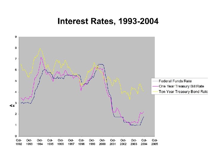
Many Bonds and Many Bond Markets, cont’d • How do changes in the Fed Funds rate affect mortgage rates or other interest rates in the economy? – The Fed Funds rate and the 1 -year Treasury bill rate move together. Why? (Hint: how do banks decide how much to charge for Fed Funds loans? how does the Fed control the Fed Funds rate? ) – The Fed Funds rate and the 1 -year T-bill rate do not move so closely with the 10 -year Treasury bond rate. Why not? • Term structure: generally, but not always, long term bonds pay higher interest rates than short term bonds. Long and short term bonds are therefore only partial substitutes for one another. Long term bonds carry greater risks of price fluctuations. Why do price fluctuations matter? • Bonds issued by different entities (government entities like cities and special purpose entities, private companies) carry different risks of default and are therefore also partial substitutes for one another. • Since bonds of various terms and default risk are partial substitutes, the Federal Reserve can reasonably hope to exercise a strong influence, if not complete control, over the whole spectrum of interest rates. But not always.