Lecture 13 Continuous Time Markov Chains Topics

Lecture 13 – Continuous. Time Markov Chains Topics • Markovian property • Exponential distribution • Rate matrix • ATM Example • Birth and death processes • Queuing systems

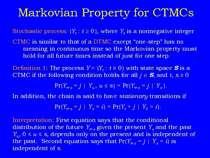Markovian Property for CTMCs Stochastic process: {Yt : t 0 }, where Yt is a nonnegative integer CTMC is similar to that of a DTMC except “one-step” has no meaning in continuous time so the Markovian property must hold for all future times instead of just for one step. Definition 1: The process Y = {Yt : t ≥ 0 } with state space S is a CTMC if the following condition holds for all j Î S, and t, s ≥ 0 Pr{Yt+s = j | Yu , u ≤ s } = Pr{Yt+s = j | Ys }. In addition, the chain is said to have stationary transitions if Pr{Yt+s = j | Ys = i } = Pr{Yt = j | Y 0 = i }. Interpretation: First equation says that the conditional distribution of the future Yt+s given the present Ys and the past Yu, 0 ≤ u ≤ s, depends only on the present and is independent of the past. Second equation says that Pr{Yt+s = j | Ys = i } is independent of s.

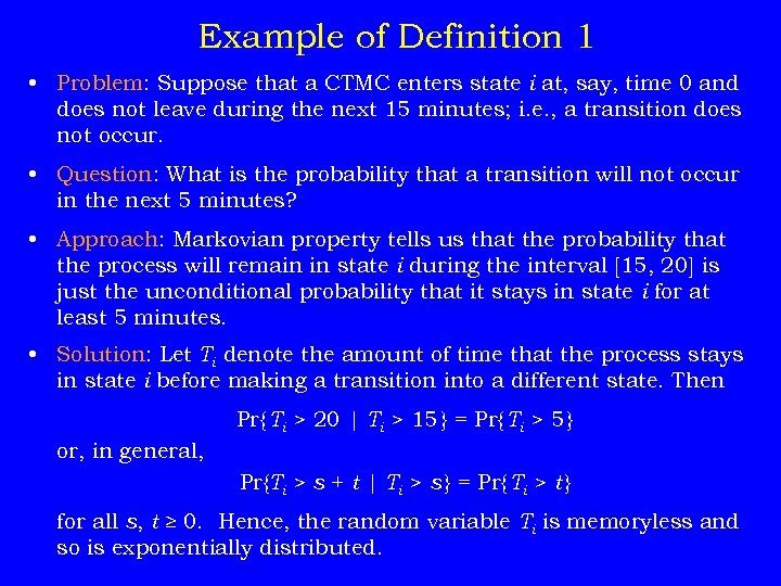Example of Definition 1 • Problem: Suppose that a CTMC enters state i at, say, time 0 and does not leave during the next 15 minutes; i. e. , a transition does not occur. • Question: What is the probability that a transition will not occur in the next 5 minutes? • Approach: Markovian property tells us that the probability that the process will remain in state i during the interval [15, 20] is just the unconditional probability that it stays in state i for at least 5 minutes. • Solution: Let Ti denote the amount of time that the process stays in state i before making a transition into a different state. Then Pr{ Ti > 20 | Ti > 15 } = Pr{ Ti > 5 } or, in general, Pr{Ti > s + t | Ti > s } = Pr{ Ti > t } for all s, t ≥ 0. Hence, the random variable Ti is memoryless and so is exponentially distributed.

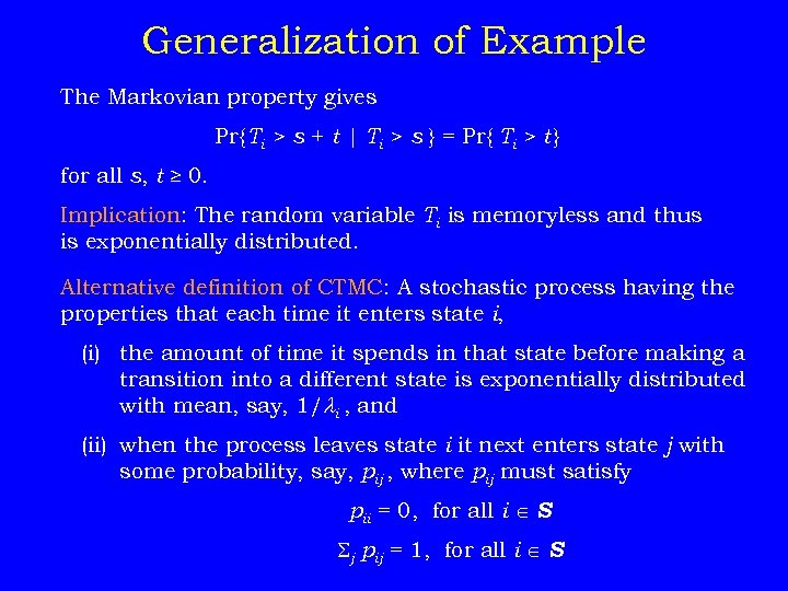Generalization of Example The Markovian property gives Pr{ Ti > s + t | Ti > s } = Pr{ Ti > t } for all s, t ≥ 0. Implication: The random variable Ti is memoryless and thus is exponentially distributed. Alternative definition of CTMC: A stochastic process having the properties that each time it enters state i, (i) the amount of time it spends in that state before making a transition into a different state is exponentially distributed with mean, say, 1/ i , and (ii) when the process leaves state i it next enters state j with some probability, say, pij , where pij must satisfy pii = 0, for all i Î S Sj pij = 1, for all i Î S

ATM Example (max of 5 in system) Statistics • Average time between arrivals = 30 sec (0. 5 min): = 2/min • Average service time = 24 sec (0. 4 min): = 2. 5/min Design questions • How many ATMs should there be? • Should the foyer be expanded? State-transition network

Exponential Distribution pdf: f (t ) = e– t for t ≥ 0 CDF: F (t ) = 1 – e– t for t ≥ 0 Parameters: Mean = 1/ Var = (1/ )2 Exponential distribution with Mean = 0. 5 ( = 2)

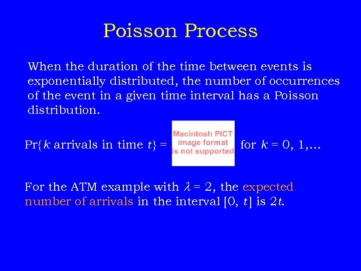Poisson Process When the duration of the time between events is exponentially distributed, the number of occurrences of the event in a given time interval has a Poisson distribution. Pr{ k arrivals in time t } = for k = 0, 1, … For the ATM example with = 2, the expected number of arrivals in the interval [0, t ] is 2 t.

Rate Diagram • For CTMCs, activities are better represented by their rate of occurrence, so rather than using a state-transition network we use a rate diagram or rate network. • This network is easily constructed from the state-transition network by replacing the activity designation by the activity rate. ATM Network Transient analysis

Rate Matrix A computationally more convenient alternative to the rate diagram is the rate matrix R whose element rij is the transition rate from state i to j. In general, rij = pij or rij = pij General rate matrix Rate matrix for ATM example

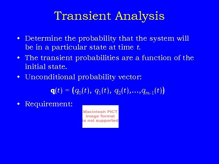Transient Analysis • Determine the probability that the system will be in a particular state at time t. • The transient probabilities are a function of the initial state. • Unconditional probability vector: q(t ) = (q 0(t ), q 1(t ), q 2(t ), …, qm-1(t )) • Requirement:

Transient Analysis (cont’d) • For some small interval of time ∆, let n = t/∆ be the number of steps or increments required to represent t. • The transient solution of the process can be approximated at time t = n∆ with a DTMC by solving the following equation: q(n∆) = q(0)P(n) or q(n∆+∆) = q(n∆)P where P is a state-transition matrix determined from the rate matrix R.

Transition Matrix for Transient Analysis Let ai be the sum of all transition rates out of state i ; that is, and let pij rij. Then

Transition Matrix for ATM Example Rate network

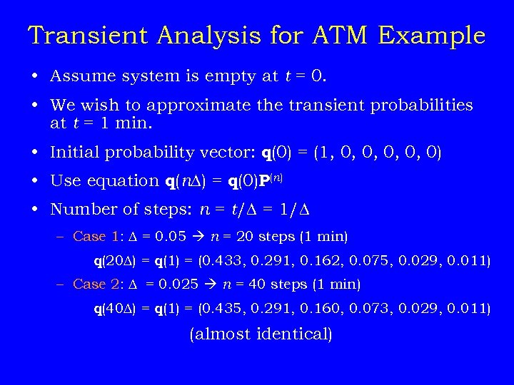Transient Analysis for ATM Example • Assume system is empty at t = 0. • We wish to approximate the transient probabilities at t = 1 min. • Initial probability vector: q(0) = (1, 0, 0, 0) • Use equation q(n∆) = q(0)P(n) • Number of steps: n = t/∆ = 1/∆ – Case 1: ∆ = 0. 05 n = 20 steps (1 min) q(20∆) = q(1) = (0. 433, 0. 291, 0. 162, 0. 075, 0. 029, 0. 011) – Case 2: ∆ = 0. 025 n = 40 steps (1 min) q(40∆) = q(1) = (0. 435, 0. 291, 0. 160, 0. 073, 0. 029, 0. 011) (almost identical)

Transient Solution for ATM Example (∆ = 0. 05, 0 t 1)

Steady-State Solutions • Definition: The probability that the system is in state i is constant (independent of initial conditions). • Steady-state probability for state i : i. P = limt q(t ) • Vector: • Calculations in Chapter 15: must solve m simultaneous linear equations in m unknowns. • ATM example: – After 1 min with ∆ = 0. 25 q(1) = (0. 435, 0. 291, 0. 160, 0. 073, 0. 029, 0. 011) – In the limit P = (0. 271, 0. 217, 0. 173, 0. 139, 0. 111, 0. 089)

Transient Computations for ATM Example with ∆ = 0. 025

System Statistics • Provide managerial insights • Evaluate system performance and quality of service • Evaluate design options • ATM Example: – Proportion of time ATM is idle: – Efficiency (proportion of time busy): – Proportion of customers rejected: – Proportion of customers who wait: – Expected number in system:

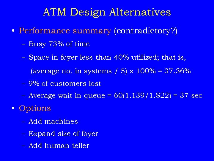
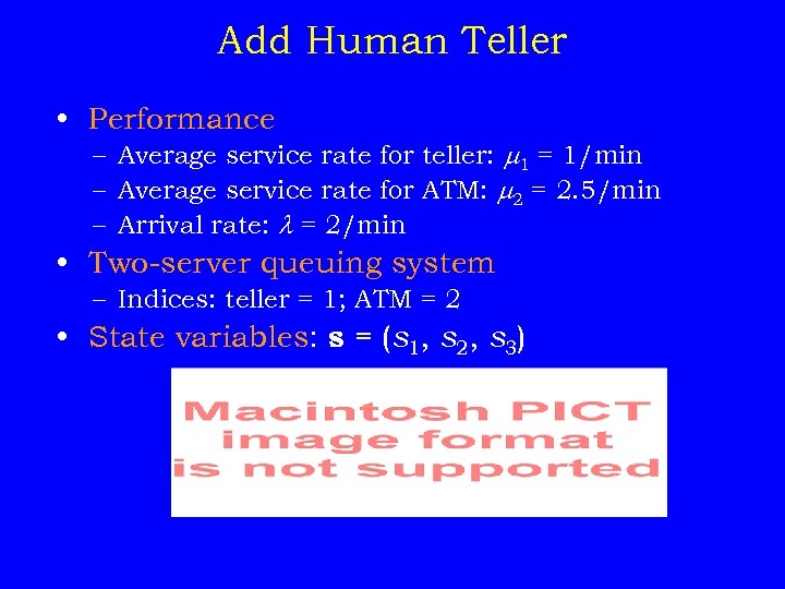
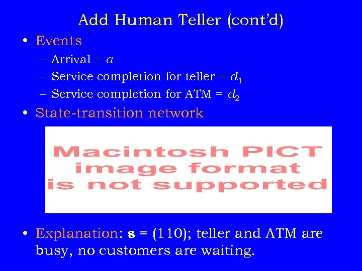
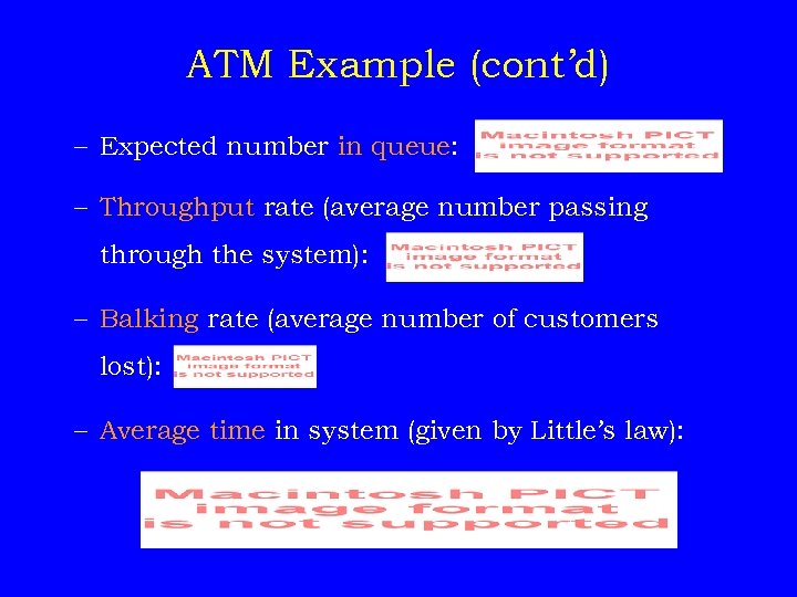ATM Example (cont’d) – Expected number in queue: – Throughput rate (average number passing through the system): – Balking rate (average number of customers lost): – Average time in system (given by Little’s law):

ATM Design Alternatives • Performance summary (contradictory? ) – Busy 73% of time – Space in foyer less than 40% utilized; that is, (average no. in systems / 5) 100% = 37. 36% – 9% of customers lost – Average wait in queue = 60(1. 139/1. 822) = 37 sec • Options – Add machines – Expand size of foyer – Add human teller

Add More ATMs Rate diagram for 3 ATMs: = 2, = 2. 5 Comparative analysis

Add Human Teller • Performance – Average service rate for teller: 1 = 1/min – Average service rate for ATM: 2 = 2. 5/min – Arrival rate: = 2/min • Two-server queuing system – Indices: teller = 1; ATM = 2 • State variables: s = (s 1, s 2, s 3)

Add Human Teller (cont’d) • Events – Arrival = a – Service completion for teller = d 1 – Service completion for ATM = d 2 • State-transition network • Explanation: s = (110); teller and ATM are busy, no customers are waiting.

Add Human Teller (cont’d) • Event rates – Arrival: = 2/min – Service completion for teller: 1 = 1 – Service completion for ATM: 2 = 2. 5 • Rate diagram

Add Human Teller (cont’d) Rate matrix R = (rij) where rij = transition rate from state i to state j Explanation: r 43 = 1 + 2. 5 = 3. 5 where state 4 = (111) and state 3 = (110)

Comparisons For ATM Example Steady-state solution for human teller: s = (000) (010) (100) (111) (112) (113) πP = (0. 214, 0. 046, 0. 313, 0. 205, 0. 117, 0. 067, 0. 038)

Pure Birth Processes Example: Hurricanes Rate matrix Properties (let i be arrival rate for state i ) • Markov process if time between arrivals has exponential distribution • No steady state [transient probabilities are governed by Poisson distribution: pk(t ) = ( t )ke- t/k !, k = 0, 1, 2, … ] • Probability of N (t ) arrivals in time t is n: Pr{ N (t ) n } =

Pure Death Processes Examples • Delivery of packages • Completion of 10 course study units Rate matrix • Let i be completion rate for state i • State space S = (0, 1, …, 10} Steady state probability vector: πP = (1, 0, …, 0) State 0 is an absorbing state

Pure Death Process Example • Assume all units have the same completion rate: rk, k– 1 = µk = µ, k = 1, …, 10 • Then transient probabilities are: p 10–k(t ) = ( t )ke- t/k !, 0 k < 10, and p 0(t ) = 1 – p 1(t ) – · · · – p 10(t ) • Let = 1 completions per week • Probability of completing k units in t = 14 weeks:

Pure Death Process Example (cont’d) • Transient probabilities for k units remaining: pk(t ) = ( t )10–ke- t/(10–k) !, 0 k < 10, and p 0(t ) = 1 – p 1(t ) – · · · – p 10(t ) • Let = 1 completions per week • Probability of k units remaining in t = 14 weeks:

General Birth and Death Processes Examples • Repair shop for a taxi company • Intensive care unit in hospital (turnover of nurses) Rate matrix • Assume 7 states • Typically, and depend on state • Steady state probabilities, P, will exist

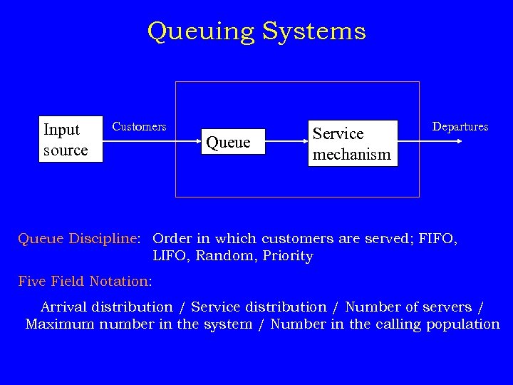Queuing Systems Input source Customers Queue Service mechanism Departures Queue Discipline: Order in which customers are served; FIFO, LIFO, Random, Priority Five Field Notation: Arrival distribution / Service distribution / Number of servers / Maximum number in the system / Number in the calling population

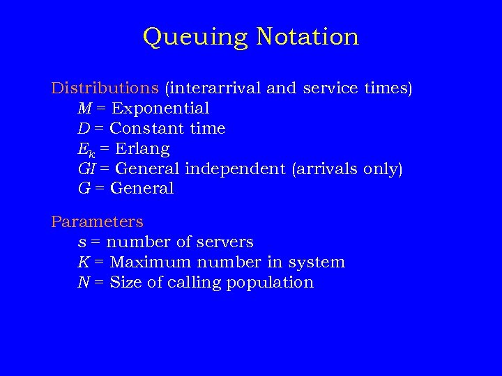Queuing Notation Distributions (interarrival and service times) M = Exponential D = Constant time Ek = Erlang GI = General independent (arrivals only) G = General Parameters s = number of servers K = Maximum number in system N = Size of calling population

Characteristics of Queues Infinite queue: e. g. , Mail order company (GI/G/s) Finite queue: e. g. , Airline reservation system (M/M/s/K) a. Customer arrives but then leaves b. No more arrivals after K

Characteristics of Queues (continued) Finite input source: e. g. , Repair shop for taxi company (N vehicles) with s service bays and limited capacity parking lot (K – s spaces). Each repair takes 1 day (GI/D/s/K/N). In this diagram N = K so we have GI/D/s/K/K system.

Single Channel Queue – Two Kinds of Service Bank teller: normal service (d ), travelers checks (c ), idle (i ) Let p = portion of customers who buy travelers checks after normal service s 1 = number in system, where s 1 Î { 0, 1, 2, . . . } s 2 = status of teller, where s 2 Î {i, d, c } s = (s 1, s 2) Statetransition network

Single Channel Queue for Bank (cont’d) • State transitions w. r. t. customer departures from teller – Current state: s = ( j, d ), j = 1, 2, … (teller busy) – Next state: either s' = ( j – 1, d ), departure with probability 1 – p, or s' = ( j, c ), get checks with probability p • State transitions w. r. t. customer departures after purchasing travelers checks – Current state: s = ( j, c ), j = 1, 2, … (customer buying checks) – Next state: s' = ( j – 1, d ), departure with probability 1 • State transitions w. r. t. customer arrivals – Current state: s = ( j, d or c), j = 1, 2, … (teller or checks busy) – Next state: s' = ( j +1, d or c), arrival with probability 1

Single Channel Queue for Bank (cont’d) • Rate of transitions – – Event: x (arrival or departure) Rate of event x : gx (where ga = , gd = 1, gc = 2) Conditional probability: p(s, s' | x ) or p(i, j|x ) Computations: rij = gxp(i, j |x ) • States -- assume limited no. customers at teller: K = 2 s 0 = (0, i ), s 1 = (1, d ), s 2 = (1, c ), s 3 = (2, d ), s 4 = (2, c ) • Rate matrix

Part Processing with Rework • Consider a machining operation in which there is a 0. 4 probability that upon completion, a processed part will not be within tolerance. • Machine is in one of 3 states [ s = { (0), (1), (2) } ]: 0 = idle 1 = working on part for first time 2 = reworking part Events a = arrival d 1 = service completion from state 1 d 2 = service completion from state 2 State-transition network

Classification of States Accessible: Possible to go from state i to state j (path exists in the network from i to j). Two states communicate if both are accessible from each other. A system is irreducible if all states communicate. State i is recurrent if the system will return to it some time in the future after leaving it. If a state is not recurrent, it is transient.

What You Should Know About Markov Chains • Definition of a CTMC. • What the difference is between a DTMC and a CTMC. • What the rate matrix and rate diagram are. • What is meant by a transient solution • What is meant by a steady-state solution. • What a birth-death process is. • Classification of the various types of queuing systems.