Lecture 10 Hypothesis Testing from a previous

Lecture 10 Hypothesis Testing

from a previous lecture … Functions of a Random Variable any function of a random variable is itself a random variable

If x has distribution p(x) the y(x) has distribution p(y) = p[x(y)] dx/dy

example Let x have a uniform (white) distribution of [0, 1] p(x) 1 0 x 1 Uniform probability that x is anywhere between 0 and 1

Let y = x 2 then x=y½ p[x(y)]=1 and dx/dy=½y-½ p(y) So p(y)=½y-½ on the interval [0, 1] y

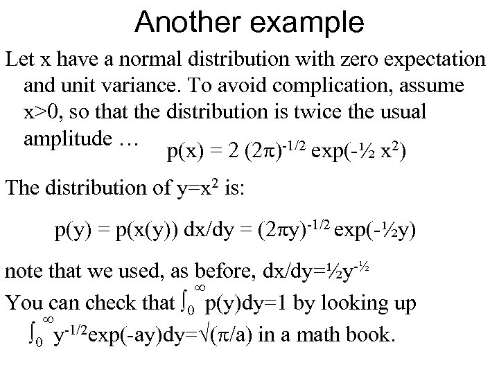Another example Let x have a normal distribution with zero expectation and unit variance. To avoid complication, assume x>0, so that the distribution is twice the usual amplitude … p(x) = 2 (2 p)-1/2 exp(-½ x 2) The distribution of y=x 2 is: p(y) = p(x(y)) dx/dy = (2 py)-1/2 exp(-½y) note that we used, as before, dx/dy=½y-½ You can check that 0 p(y)dy=1 by looking up 0 y-1/2 exp(-ay)dy= (p/a) in a math book.

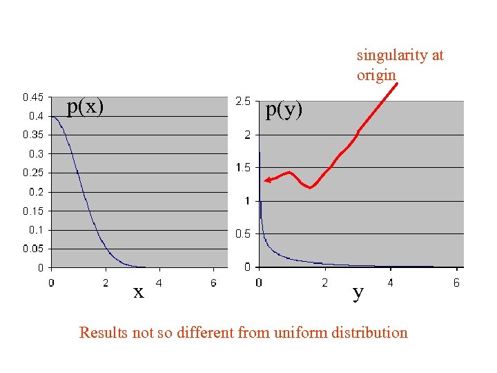singularity at origin p(x) p(y) x y Results not so different from uniform distribution

from a previous lecture … Functions of Two Random Variables any function of a several random variables is itself a random variable

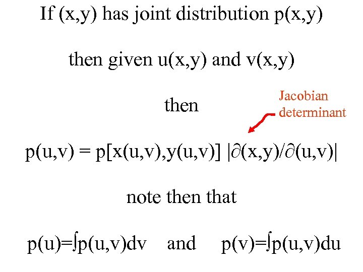If (x, y) has joint distribution p(x, y) then given u(x, y) and v(x, y) then Jacobian determinant p(u, v) = p[x(u, v), y(u, v)] | (x, y)/ (u, v)| note then that p(u)= p(u, v)dv and p(v)= p(u, v)du

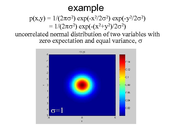example p(x, y) = 1/(2 ps 2) exp(-x 2/2 s 2) exp(-y 2/2 s 2) = 1/(2 ps 2) exp(-(x 2+y 2)/2 s 2) uncorrelated normal distribution of two variables with zero expectation and equal variance, s s=1

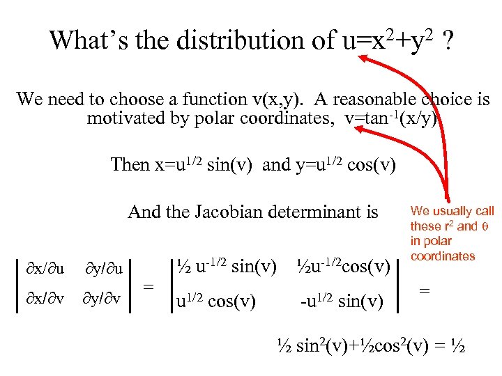What’s the distribution of u=x 2+y 2 ? We need to choose a function v(x, y). A reasonable choice is motivated by polar coordinates, v=tan-1(x/y) Then x=u 1/2 sin(v) and y=u 1/2 cos(v) And the Jacobian determinant is x/ u y/ u x/ v y/ v = ½ u-1/2 sin(v) ½u-1/2 cos(v) u 1/2 cos(v) -u 1/2 sin(v) We usually call these r 2 and q in polar coordinates = s=1 ½ sin 2(v)+½cos 2(v) = ½

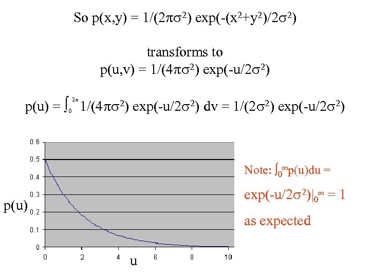So p(x, y) = 1/(2 ps 2) exp(-(x 2+y 2)/2 s 2) transforms to p(u, v) = 1/(4 ps 2) exp(-u/2 s 2) p(u) = 0 1/(4 ps 2) exp(-u/2 s 2) dv = 1/(2 s 2) exp(-u/2 s 2) 2 p Note: 0 p(u)du = exp(-u/2 s 2)|0 = 1 p(u) as expected u

The point of my showing you this is to give you the sense that computing the probability distributions associated with functions of random variables is not particularly mysterious but instead is rather routine (though possibly algebraically tedious)

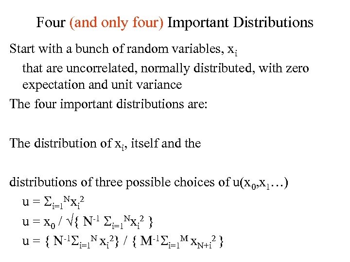Four (and only four) Important Distributions Start with a bunch of random variables, xi that are uncorrelated, normally distributed, with zero expectation and unit variance The four important distributions are: The distribution of xi, itself and the distributions of three possible choices of u(x 0, x 1…) u = Si=1 Nxi 2 u = x 0 / { N-1 Si=1 Nxi 2 } u = { N-1 Si=1 N xi 2} / { M-1 Si=1 M x. N+i 2 }

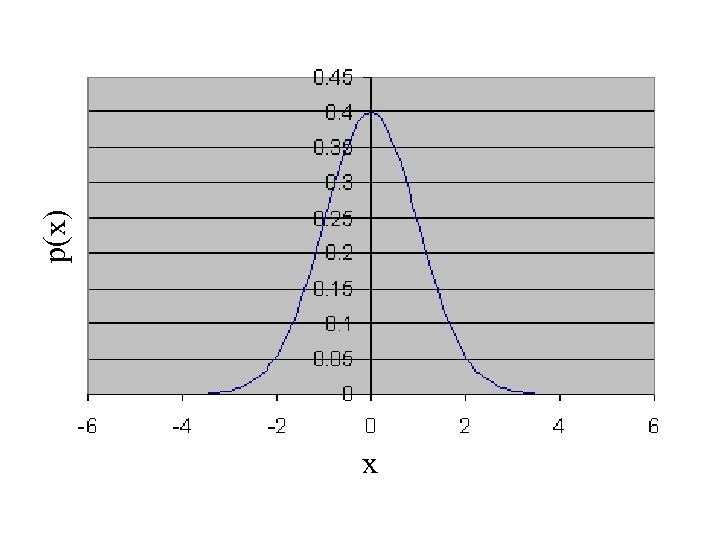
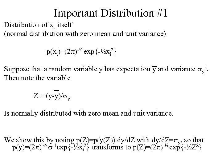Important Distribution #1 Distribution of xi itself (normal distribution with zero mean and unit variance) p(xi)=(2 p)-½ exp{-½xi 2} Suppose that a random variable y has expectation y and variance sy 2. Then note the variable Z = (y-y)/sy Is normally distributed with zero mean and unit variance. We show this by noting p(Z)=p(y(Z)) dy/d. Z with dy/d. Z=sy, so that p(y)=(2 p)-½ s-1 exp{-½xi 2} transforms to p(Z)=(2 p)-½ exp{-½Z 2}

x p(x)

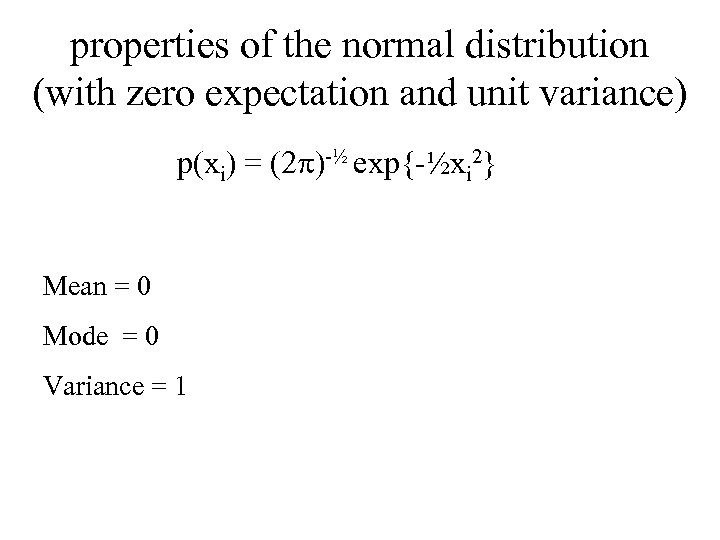properties of the normal distribution (with zero expectation and unit variance) p(xi) = (2 p)-½ exp{-½xi 2} Mean = 0 Mode = 0 Variance = 1

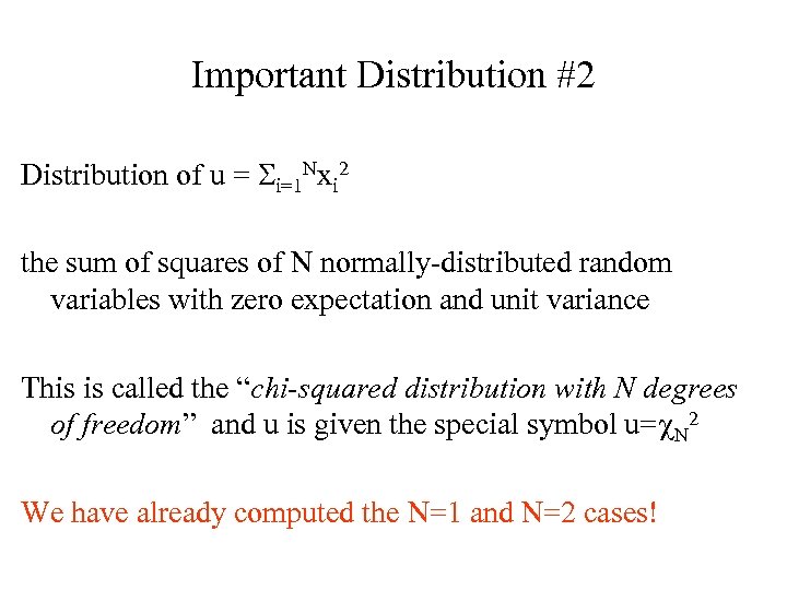Important Distribution #2 Distribution of u = Si=1 Nxi 2 the sum of squares of N normally-distributed random variables with zero expectation and unit variance This is called the “chi-squared distribution with N degrees of freedom” and u is given the special symbol u=c. N 2 We have already computed the N=1 and N=2 cases!

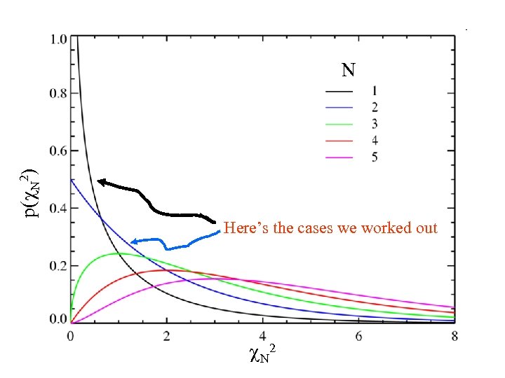p(c. N 2) N Here’s the cases we worked out c N 2

properties of the chi-squared distribution 1 2) = [c 2]½N-1 exp{ -½ [c 2] } p(c. N N N 2½N (½N-1)! Mean = N Mode = 0 if N<2 N-2 otherwise Variance = 2 N

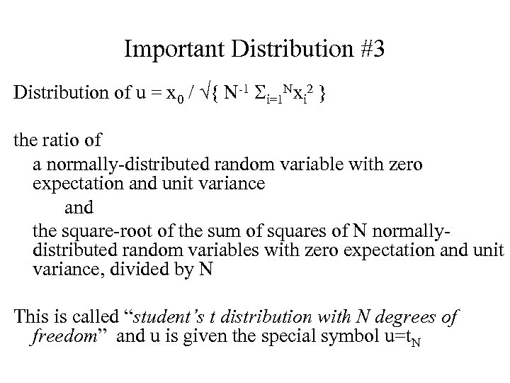Important Distribution #3 Distribution of u = x 0 / { N-1 Si=1 Nxi 2 } the ratio of a normally-distributed random variable with zero expectation and unit variance and the square-root of the sum of squares of N normallydistributed random variables with zero expectation and unit variance, divided by N This is called “student’s t distribution with N degrees of freedom” and u is given the special symbol u=t. N

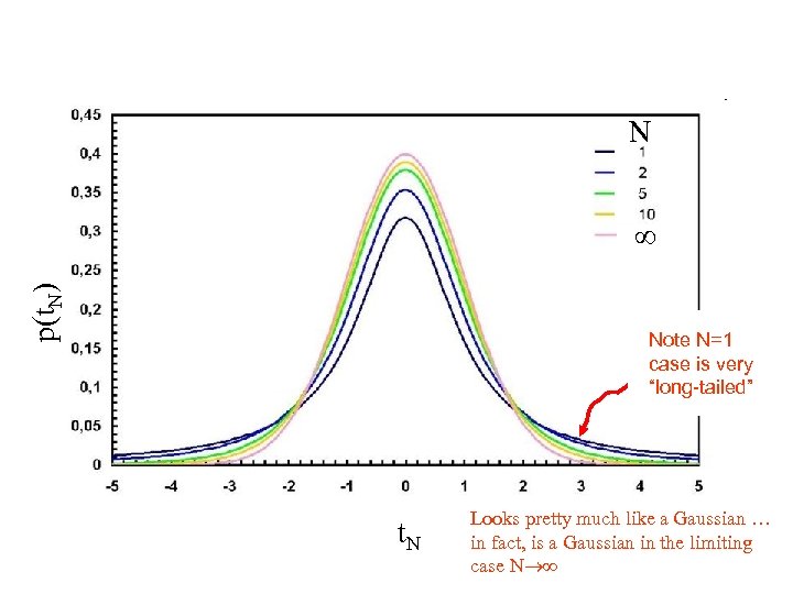N p(t. N) Note N=1 case is very “long-tailed” t. N Looks pretty much like a Gaussian … in fact, is a Gaussian in the limiting case N

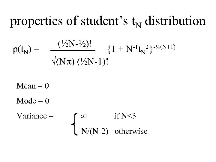properties of student’s t. N distribution (½N-½)! p(t. N) = {1 + N-1 t. N 2}-½(N+1) (Np) (½N-1)! Mean = 0 Mode = 0 Variance = if N<3 N/(N-2) otherwise

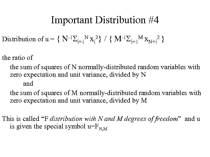Important Distribution #4 Distribution of u = { N-1 Si=1 N xi 2} / { M-1 Si=1 M x. N+i 2 } the ratio of the sum of squares of N normally-distributed random variables with zero expectation and unit variance, divided by N and the sum of squares of M normally-distributed random variables with zero expectation and unit variance, divided by M This is called “F distribution with N and M degrees of freedom” and u is given the special symbol u=FN, M

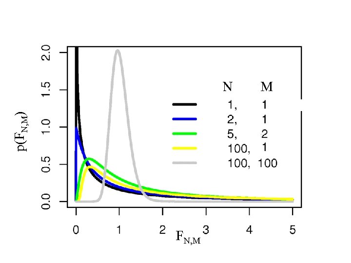p(FN, M) N FN, M M

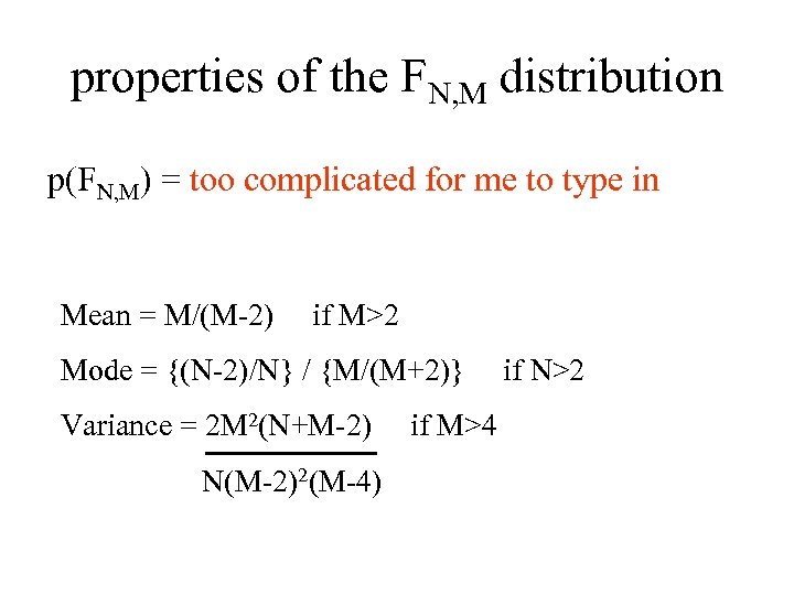properties of the FN, M distribution p(FN, M) = too complicated for me to type in Mean = M/(M-2) if M>2 Mode = {(N-2)/N} / {M/(M+2)} if N>2 Variance = 2 M 2(N+M-2) if M>4 N(M-2)2(M-4)

Hypothesis Testing

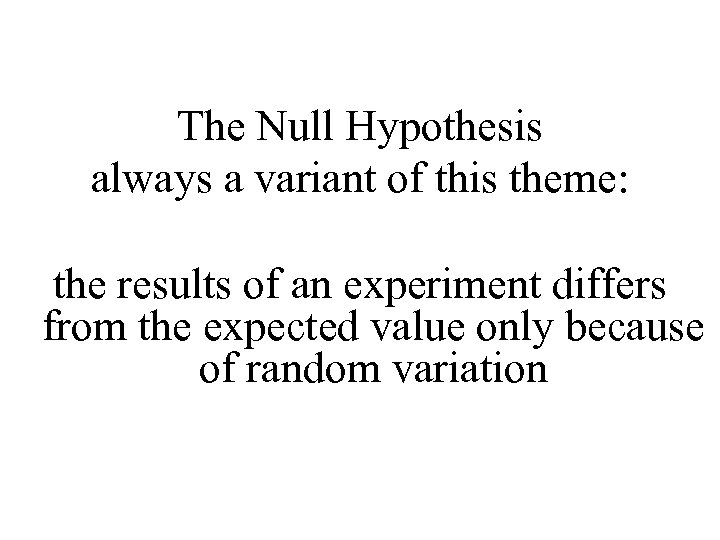The Null Hypothesis always a variant of this theme: the results of an experiment differs from the expected value only because of random variation

Test of Significance of Results say to 95% significance The Null Hypothesis would generate the observed result less than 5% of the time

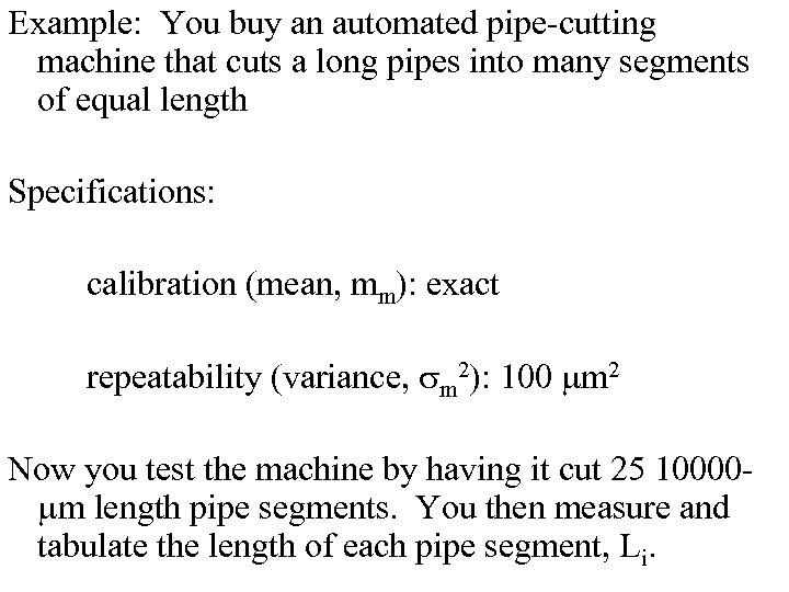Example: You buy an automated pipe-cutting machine that cuts a long pipes into many segments of equal length Specifications: calibration (mean, mm): exact repeatability (variance, sm 2): 100 mm 2 Now you test the machine by having it cut 25 10000 mm length pipe segments. You then measure and tabulate the length of each pipe segment, Li.

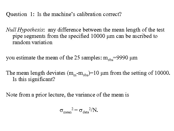Question 1: Is the machine’s calibration correct? Null Hypothesis: any difference between the mean length of the test pipe segments from the specified 10000 mm can be ascribed to random variation you estimate the mean of the 25 samples: mobs=9990 mm The mean length deviates (mm-mobs)=10 mm from the setting of 10000. Is this significant? Note from a prior lecture, the variance of the mean is smean 2 = sdata 2/N.

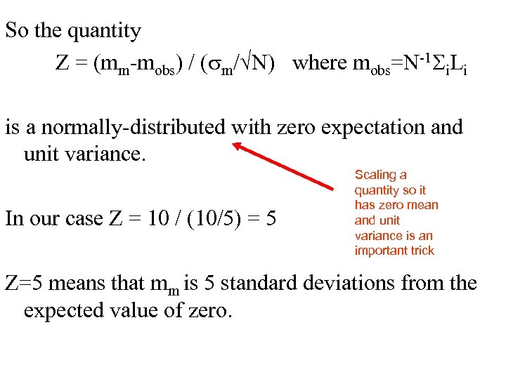So the quantity Z = (mm-mobs) / (sm/ N) where mobs=N-1 Si. Li is a normally-distributed with zero expectation and unit variance. In our case Z = 10 / (10/5) = 5 Scaling a quantity so it has zero mean and unit variance is an important trick Z=5 means that mm is 5 standard deviations from the expected value of zero.

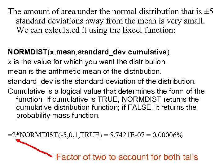The amount of area under the normal distribution that is ± 5 standard deviations away from the mean is very small. We can calculated it using the Excel function: NORMDIST(x, mean, standard_dev, cumulative) x is the value for which you want the distribution. mean is the arithmetic mean of the distribution. standard_dev is the standard deviation of the distribution. Cumulative is a logical value that determines the form of the function. If cumulative is TRUE, NORMDIST returns the cumulative distribution function; if FALSE, it returns the probability mass function. =2*NORMDIST(-5, 0, 1, TRUE) = 5. 7421 E-07 = 0. 00006% Factor of two to account for both tails

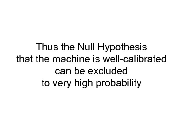Thus the Null Hypothesis that the machine is well-calibrated can be excluded to very high probability

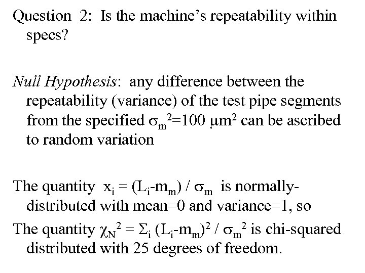Question 2: Is the machine’s repeatability within specs? Null Hypothesis: any difference between the repeatability (variance) of the test pipe segments from the specified sm 2=100 mm 2 can be ascribed to random variation The quantity xi = (Li-mm) / sm is normallydistributed with mean=0 and variance=1, so The quantity c. N 2 = Si (Li-mm)2 / sm 2 is chi-squared distributed with 25 degrees of freedom.

Suppose that the root mean squared variation of pipe lengths was [N-1 Si (Li-mm)2]½ = 12 mm. Then c 252 = Si (Li-mm)2 / sm 2 = 25 144 / 100 = 36 CHIDIST(x, degrees_freedom) x is the value at which you want to evaluate the distribution. degrees_freedom is the number of degrees of freedom. CHIDIST = P(X>x), where X is a y 2 random variable. The probability that c 252 36 is CHIDIST(36, 25)=0. 07 or 7%

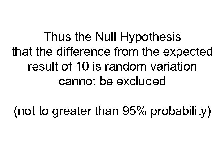Thus the Null Hypothesis that the difference from the expected result of 10 is random variation cannot be excluded (not to greater than 95% probability)

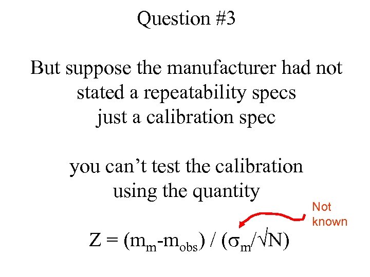Question #3 But suppose the manufacturer had not stated a repeatability specs just a calibration spec you can’t test the calibration using the quantity Z = (mm-mobs) / (sm/ N) Not known

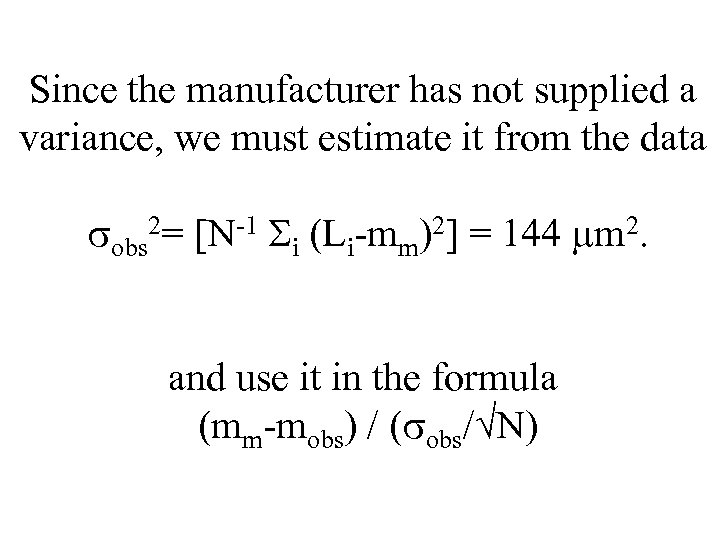Since the manufacturer has not supplied a variance, we must estimate it from the data sobs 2= [N-1 Si (Li-mm)2] = 144 mm 2. and use it in the formula (mm-mobs) / (sobs/ N)

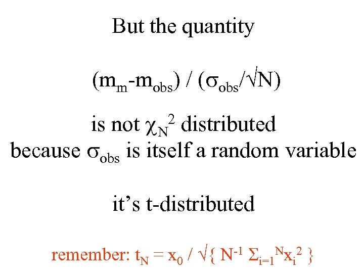But the quantity (mm-mobs) / (sobs/ N) is not c. N 2 distributed because sobs is itself a random variable it’s t-distributed remember: t. N = x 0 / { N-1 Si=1 Nxi 2 }

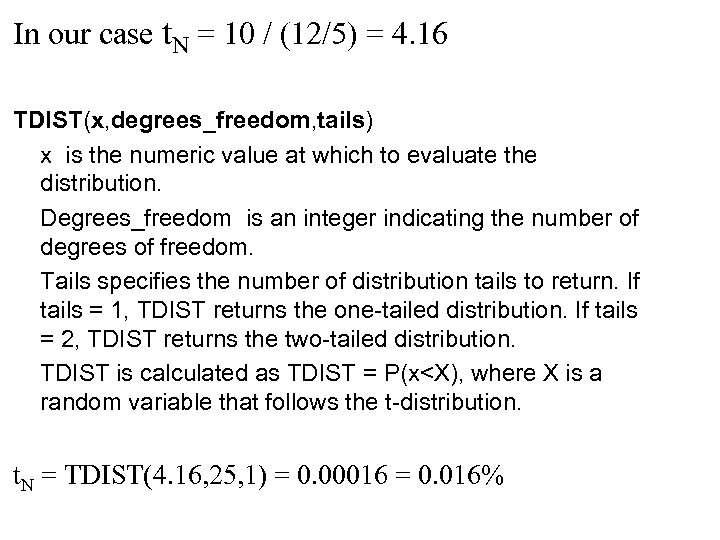In our case t. N = 10 / (12/5) = 4. 16 TDIST(x, degrees_freedom, tails) x is the numeric value at which to evaluate the distribution. Degrees_freedom is an integer indicating the number of degrees of freedom. Tails specifies the number of distribution tails to return. If tails = 1, TDIST returns the one-tailed distribution. If tails = 2, TDIST returns the two-tailed distribution. TDIST is calculated as TDIST = P(x

Thus the Null Hypothesis that the difference from the expected result of 10000 is due to random variation can be excluded to high probability, but not nearly has high as when the manufacturer told us the repeatability

Question #4 Suppose you performed the test twice, a year apart, and wanted to know has the repeatability changed? This Year: [N-1 Si (Lyr 1 i-mm)2]½ = 12 mm Last Year: [M-1 Si (Lyr 2 i-mm)2]½ = 14 mm (lets say N=M=25 in both cases)

Null Hypothesis: any difference between the repeatability (variance) of the test pipe segments between years can be ascribed to random variation The ratio of mean-squared error is F-distributed FN, M = { N-1 Si=1 N xi 2} / { M-1 Si=1 M x. N+i 2 } = 12/14 = 0. 857

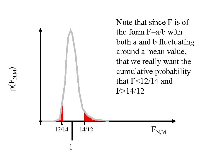p(FN, M) Note that since F is of the form F=a/b with both a and b fluctuating around a mean value, that we really want the cumulative probability that F<12/14 and F>14/12 12/14 14/12 1 FN, M

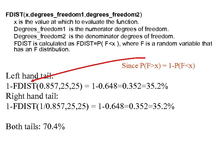FDIST(x, degrees_freedom 1, degrees_freedom 2) x is the value at which to evaluate the function. Degrees_freedom 1 is the numerator degrees of freedom. Degrees_freedom 2 is the denominator degrees of freedom. FDIST is calculated as FDIST=P( Fx) = 1 -P(F

Thus the Null Hypothesis that the year-to-year difference in variance is due to random variation cannot be excluded there is no strong reason to believe that the repeatability of the machine has changed between the years

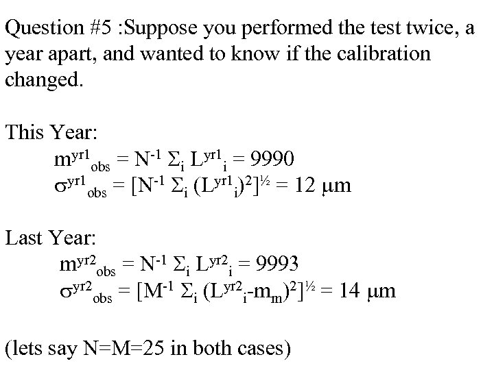Question #5 : Suppose you performed the test twice, a year apart, and wanted to know if the calibration changed. This Year: myr 1 obs = N-1 Si Lyr 1 i = 9990 syr 1 obs = [N-1 Si (Lyr 1 i)2]½ = 12 mm Last Year: myr 2 obs = N-1 Si Lyr 2 i = 9993 syr 2 obs = [M-1 Si (Lyr 2 i-mm)2]½ = 14 mm (lets say N=M=25 in both cases)

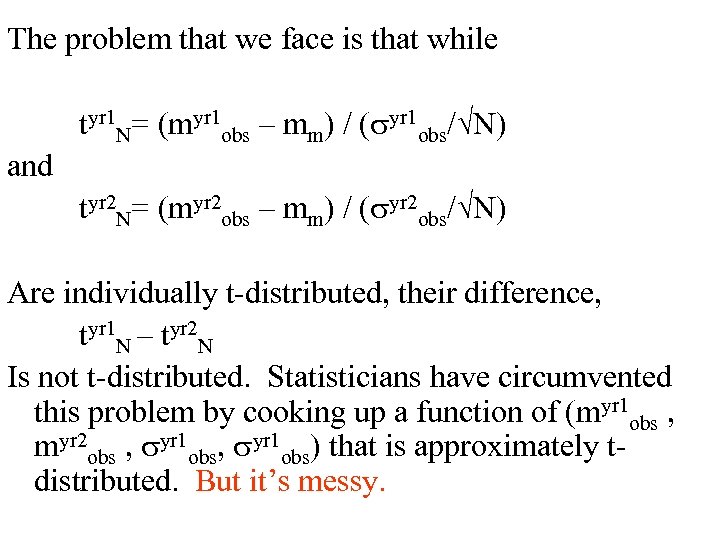The problem that we face is that while tyr 1 N= (myr 1 obs – mm) / (syr 1 obs/ N) and tyr 2 N= (myr 2 obs – mm) / (syr 2 obs/ N) Are individually t-distributed, their difference, tyr 1 N – tyr 2 N Is not t-distributed. Statisticians have circumvented this problem by cooking up a function of (myr 1 obs , myr 2 obs , syr 1 obs) that is approximately tdistributed. But it’s messy.

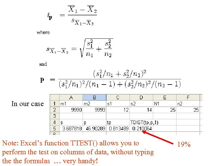In our case Note: Excel’s function TTEST() allows you to perform the test on columns of data, without typing the formulas … very handy! 19%

Thus the Null Hypothesis that the difference in means is due to random variation cannot be excluded

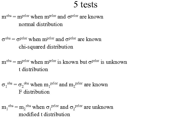5 tests mobs = mprior when mprior and sprior are known normal distribution sobs = sprior when mprior and sprior are known chi-squared distribution mobs = mprior when mprior is known but sprior is unknown t distribution s 1 obs = s 2 obs when m 1 prior and m 2 prior are known F distribution m 1 obs = m 2 obs when s 1 prior and s 2 prior are unknown modified t distribution

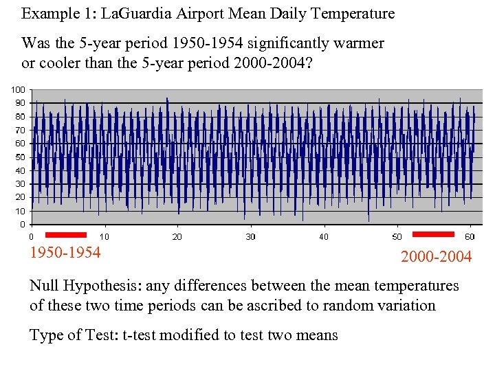Example 1: La. Guardia Airport Mean Daily Temperature Was the 5 -year period 1950 -1954 significantly warmer or cooler than the 5 -year period 2000 -2004? 1950 -1954 2000 -2004 Null Hypothesis: any differences between the mean temperatures of these two time periods can be ascribed to random variation Type of Test: t-test modified to test two means

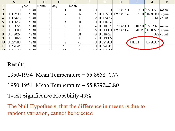Results 1950 -1954 Mean Temperature = 55. 8658± 0. 77 1950 -1954 Mean Temperature = 55. 8792± 0. 80 T-test Significance Probability 49% The Null Hypothesis, that the difference in means is due to random variation, cannot be rejected

Issue about noise Note that we are estimating s by treating the short-term (days-tomonths) temperature fluctuations as ‘noise’ Is this correct? Certainly such fluctuations are not measurement noise in the normal sense. They might be considered ‘model noise’ in the sense that they are caused by weather systems that are unmodeled (by us) However, such noise probably does not meet all the requirements for use in the statistical test. In particular, it probably has some day-to-day correlation (hot today, hot tomorrow, too) that violated our implicit assumption of uncorrelated noise.

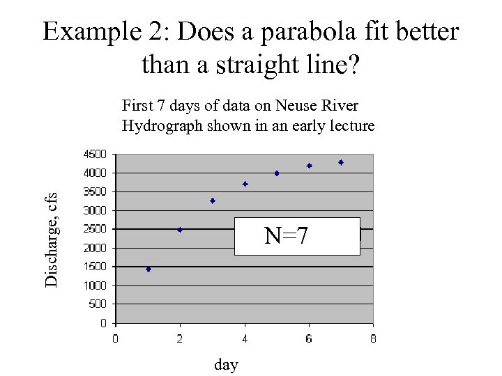Example 2: Does a parabola fit better than a straight line? Discharge, cfs First 7 days of data on Neuse River Hydrograph shown in an early lecture N=7 day

A parabola will always fit better than a straight line because it has an extra parameter But does it fit significantly better? Null Hypothesis: Any difference in fit is due to random variation

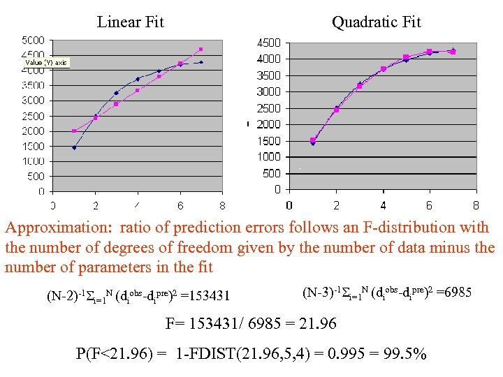Linear Fit Quadratic Fit Approximation: ratio of prediction errors follows an F-distribution with the number of degrees of freedom given by the number of data minus the number of parameters in the fit (N-2)-1 Si=1 N (diobs-dipre)2 =153431 (N-3)-1 Si=1 N (diobs-dipre)2 =6985 F= 153431/ 6985 = 21. 96 P(F<21. 96) = 1 -FDIST(21. 96, 5, 4) = 0. 995 = 99. 5%

The Null Hypothesis can be rejected with 99. 5% confidence

Another Issue about noise Note that we are again basing estimates upon ‘model noise’ in the sense that the prediction error is being controlled – at least partly - by the misfit of the curve, as well as by measurement error As before, such noise probably does not meet all the requirements for use in the statistical test. So the test needs to be used with some caution.