Lecture 1_ENG_2014.pptx
- Количество слайдов: 24
Lecture 1 Introductory Econometrics September, 6 2014
Introductory Econometrics Course Lecturer: Podvysotska Tamara Olexandrivna tpodvysotskaya@gmail. com Schedule Lectures – Saturdays: 1: 30 -2: 50 p. m. – financiers &marketing specialists, room 4 -101 • Practice Sessions – Saturdays: • 3: 00 - 4: 20 p. m. – Group #1/#2, room 6 -306 • 4: 30 -5: 50 p. m. – Group #3/#4, room 6 -306 • • •
Introductory Econometrics Course Requirements: 12 lectures 6 practice sessions (seminars) 5 home assignments (account for 30 points) Midterm Exam (account for 20 points) Written Final Exam (account for 50 points) Minimum required to pass the course: At least 30 points in the exam + 20 points Recommended literature: Лук’яненко І. Г. , Краснікова Л. І. Економетрика. Теорія та практика. К. : Знання, 1998 — 493 с. • Damodar N. Gujarati : Basic Econometrics. Mc. Graw. Hill Bool Company, 1995. - 838 р. • Wooldridge J. M. Introductory Econometrics: A Modern Approach. Thomson South-Western, 2002. – 863 p. • Колеников. С. Прикладной эконометрический анализ в статистическом пакете Stata. – РЭШ, 2000. ‑ 111 с. • • •
Course Content Lectures: • Lecture 1: Introduction, repetition of statistical background • Lectures 2 -6: Linear regression models • Lectures 7 -10: Violation of standard assumptions • Lecture 11. Introduction to qualitative dependent variables • Lecture 12. Revision Practice Sessions: • Will serve to clarify and apply concepts presented on lectures • To solve the exercises we will use statistical package STATA

What is econometrics? • To beginning students, it may seem as if econometrics is an overly complex obstacle to an otherwise useful education. (. . . ) • To professionals in the field, econometric is a fascinating set of techniques that allows the measurement and analysis of economic phenomena and the prediction of future economic trends. A. H. Studenmund (Using Econometrics: A Practical Guide)
What is Econometrics? • Econometrics is the quantitative measurement and analysis of actual economic and business phenomena • It attempts to quantify economic reality and bridge the gap between the abstract world of economic theory and the real world of human activity It has three major uses: • 1. describing economic reality • 2. testing hypotheses about economic theory • 3. forecasting future economic activity
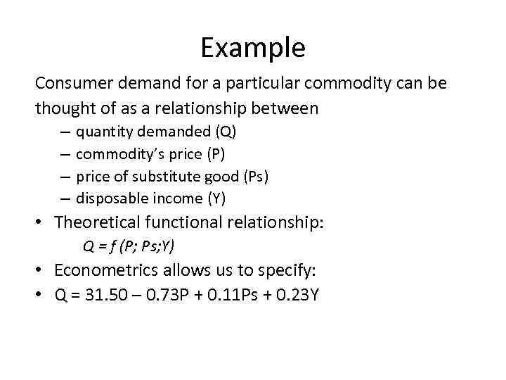
Example Consumer demand for a particular commodity can be thought of as a relationship between – – quantity demanded (Q) commodity’s price (P) price of substitute good (Ps) disposable income (Y) • Theoretical functional relationship: Q = f (P; Ps; Y) • Econometrics allows us to specify: • Q = 31. 50 – 0. 73 P + 0. 11 Ps + 0. 23 Y
Random Variables A random variable X is a variable whose numerical value is determined by chance. It is a quantification of the outcome of a random phenomenon. Discrete random variable: has a countable number of possible values Example: – the number of times that a coin will be flipped before a heads is obtained – the number of newborn girls among 100 newborn babies is a discrete random variable that can take a value 0, 1, 2, 3, 4, 5, ………, 100 Continuous random variable: can take on any value in an interval Example: – time until the first goal is shot in a football match between FC Barcelona and Real Madrid – The distance which the projectile of a fired gun would fly. It would take the values from interval (a, b)
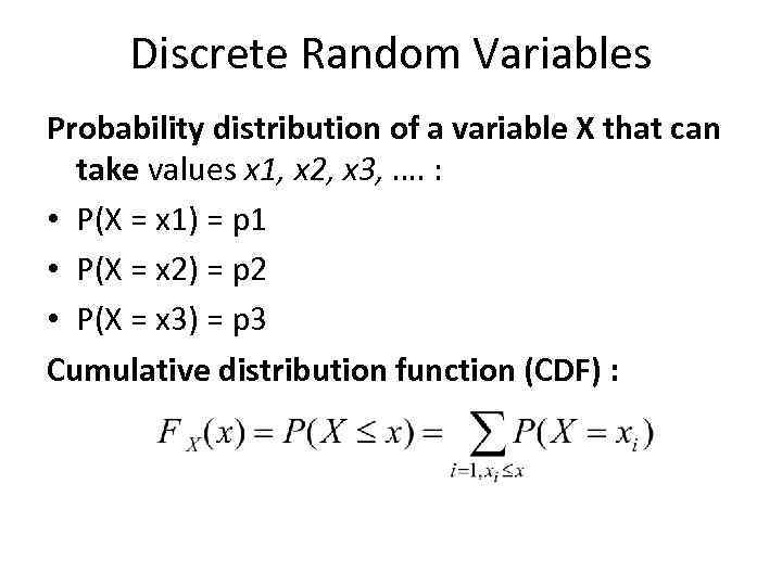
Discrete Random Variables Probability distribution of a variable X that can take values x 1, x 2, x 3, …. : • P(X = x 1) = p 1 • P(X = x 2) = p 2 • P(X = x 3) = p 3 Cumulative distribution function (CDF) :
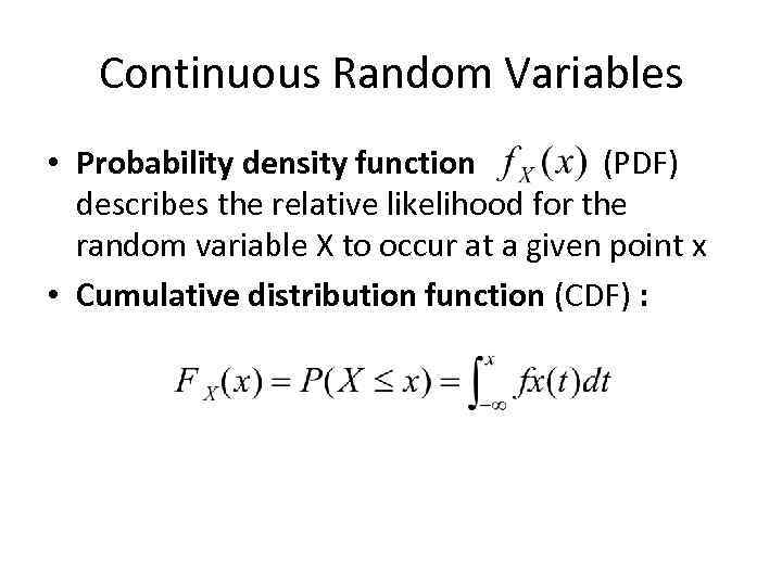
Continuous Random Variables • Probability density function (PDF) describes the relative likelihood for the random variable X to occur at a given point x • Cumulative distribution function (CDF) :
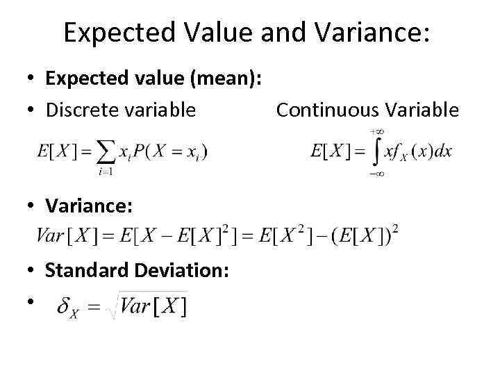
Expected Value and Variance: • Expected value (mean): • Discrete variable Continuous Variable • Variance: • Standard Deviation: •
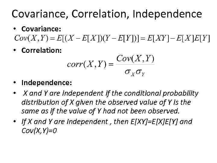
Covariance, Correlation, Independence • Covariance: • Correlation: • Independence: • X and Y are independent if the conditional probability distribution of X given the observed value of Y is the same as if the value of Y had not been observed. • If X and Y are independent , then E[XY]=E[X]E[Y] and Cov(X, Y)=0
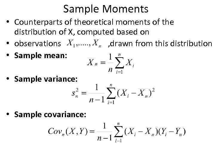
Sample Moments • Counterparts of theoretical moments of the distribution of X, computed based on • observations , drawn from this distribution • Sample mean: • Sample variance: • Sample covariance:
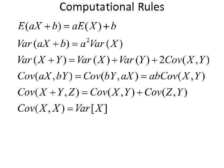
Computational Rules
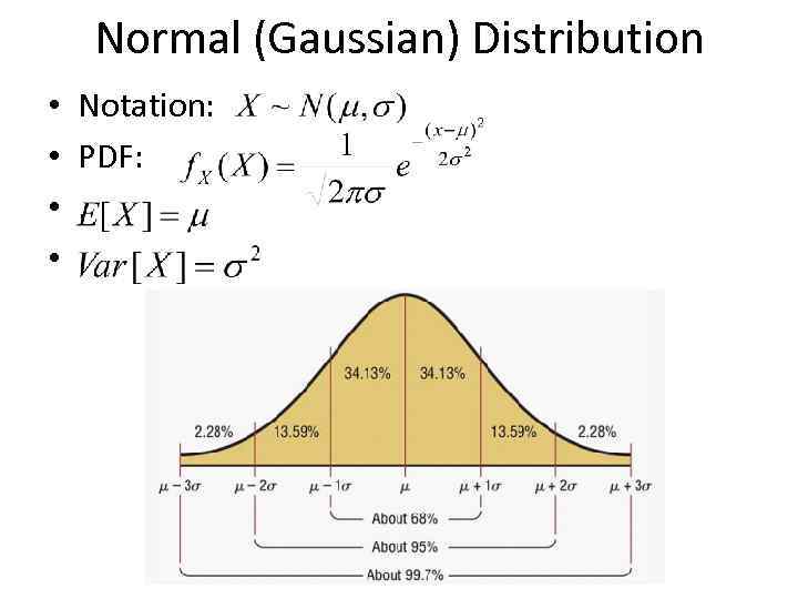
Normal (Gaussian) Distribution • • Notation: PDF: . .

Standardized Random Variable • Standardization is used for better comparison of different variables • Define Z to be the standardized variable of X: • No matter what are the expected value and variance of X, it always holds that: • and • Standard normal distribution:
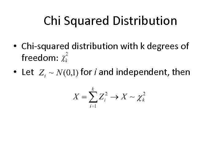
Chi Squared Distribution • Chi-squared distribution with k degrees of freedom: • Let for i and independent, then
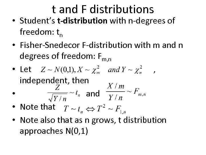
t and F distributions • Student’s t-distribution with n-degrees of freedom: tn • Fisher-Snedecor F-distribution with m and n degrees of freedom: Fm, n • Let , independent, then • and • Note that • Note also that as n grows, t distribution approaches N(0, 1)
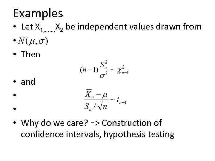
Examples • Let X 1, ……. X 2 be independent values drawn from • • Then • • and Why do we care? => Construction of confidence intervals, hypothesis testing

Some terminology • Population: the entire group of items that interests us • Sample: the part of population that we actually observe • Statistical inference: use of the sample to draw conclusion about the characteristics of the population from which the sample came • Correct statistical inference can be performed only on a random sample – a sample that reflects the true distribution of population • Biased sample – any sample that differs systematically from the population that it is intended to represent • Selection bias – occurs when the selection of the sample systematically excludes or under represents certain groups • Self-selection bias – occurs when we examine data for a group of people who have chosen to be in that group
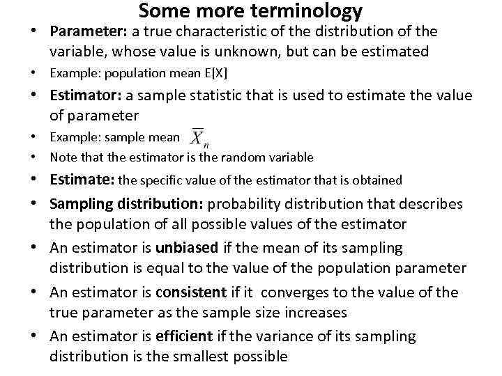
Some more terminology • Parameter: a true characteristic of the distribution of the variable, whose value is unknown, but can be estimated • Example: population mean E[X] • Estimator: a sample statistic that is used to estimate the value of parameter • Example: sample mean • Note that the estimator is the random variable • Estimate: the specific value of the estimator that is obtained • Sampling distribution: probability distribution that describes the population of all possible values of the estimator • An estimator is unbiased if the mean of its sampling distribution is equal to the value of the population parameter • An estimator is consistent if it converges to the value of the true parameter as the sample size increases • An estimator is efficient if the variance of its sampling distribution is the smallest possible
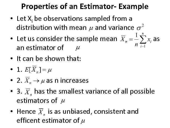
Properties of an Estimator- Example • Let Xi be observations sampled from a distribution with mean and variance • Let us consider the sample mean as an estimator of • It can be shown that: • 1. • 2. as n increases • 3. has the smallest variance of all possible estimators of • Hence is as unbiased, consistent and efficent estimator of
Summary • Today we revised some concepts from statistics that we will use throughout our econometrics classes • It was a very brief overview, serving only for information what students are expected to know already • The focus was on distributions and their moments, on sampling and estimation terminology
To be continued… • On the exercise session we will practice some of the concepts mentioned today • Work with normal distribution (tables) • Construction of confidence interval • On the next lecture we will start with regression analysis and introduce the Ordinary Least Squares (OLS) estimator
Lecture 1_ENG_2014.pptx