57aadcf35dfcb4aefb43f9900f56f385.ppt
- Количество слайдов: 29
 Lecture: 1 - Introduction How to Do Well In This Class 1. Spend enough time on the homework problems and articles so that you feel comfortable with the topic. - this does not necessarily mean you get everything correct – but complete ignorance will not be bliss when it comes time for the exam. 2. Listen and participate in class by answering and asking questions. Studies show that people remember much more of what they hear than what they read, so simply reading the notes and book may not be enough for many students. -active participation is also a better way to remember the material we cover. For those who often struggle on exams, it shows me that you may still be competent in the subject matter and are at least trying.
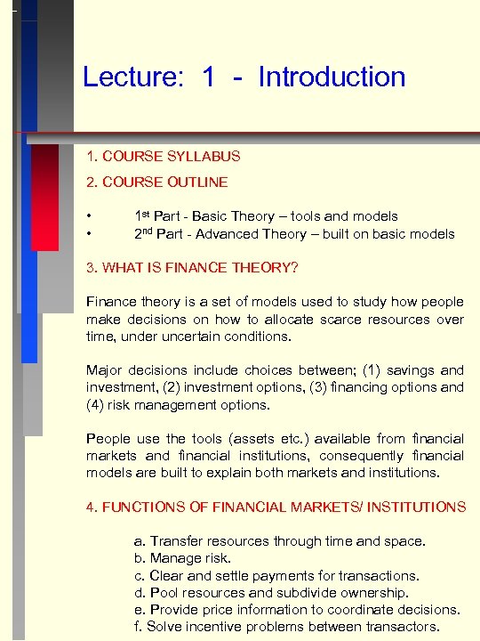 Lecture: 1 - Introduction 1. COURSE SYLLABUS 2. COURSE OUTLINE • • 1 st Part - Basic Theory – tools and models 2 nd Part - Advanced Theory – built on basic models 3. WHAT IS FINANCE THEORY? Finance theory is a set of models used to study how people make decisions on how to allocate scarce resources over time, under uncertain conditions. Major decisions include choices between; (1) savings and investment, (2) investment options, (3) financing options and (4) risk management options. People use the tools (assets etc. ) available from financial markets and financial institutions, consequently financial models are built to explain both markets and institutions. 4. FUNCTIONS OF FINANCIAL MARKETS/ INSTITUTIONS a. Transfer resources through time and space. b. Manage risk. c. Clear and settle payments for transactions. d. Pool resources and subdivide ownership. e. Provide price information to coordinate decisions. f. Solve incentive problems between transactors.
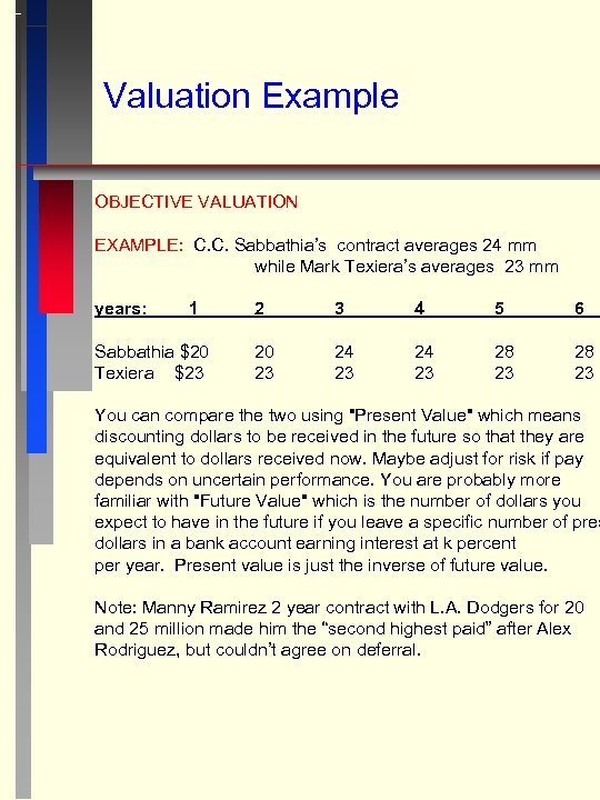 Valuation Example OBJECTIVE VALUATION EXAMPLE: C. C. Sabbathia’s contract averages 24 mm while Mark Texiera’s averages 23 mm years: 1 Sabbathia $20 Texiera $23 2 3 4 5 6 20 23 24 23 28 23 You can compare the two using "Present Value" which means discounting dollars to be received in the future so that they are equivalent to dollars received now. Maybe adjust for risk if pay depends on uncertain performance. You are probably more familiar with "Future Value" which is the number of dollars you expect to have in the future if you leave a specific number of pres dollars in a bank account earning interest at k percent per year. Present value is just the inverse of future value. Note: Manny Ramirez 2 year contract with L. A. Dodgers for 20 and 25 million made him the “second highest paid” after Alex Rodriguez, but couldn’t agree on deferral.
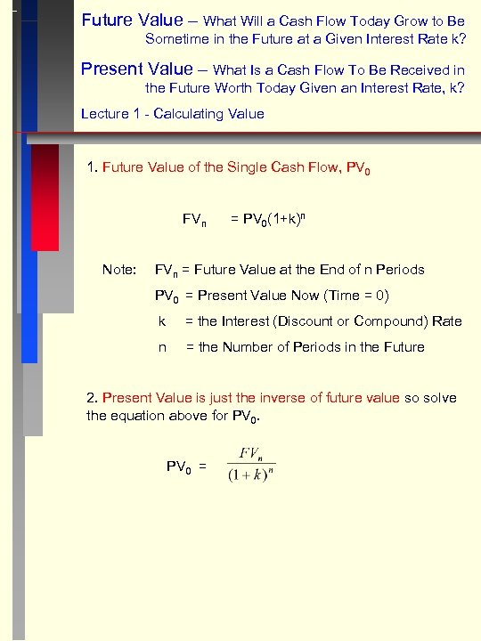 Future Value – What Will a Cash Flow Today Grow to Be Sometime in the Future at a Given Interest Rate k? Present Value – What Is a Cash Flow To Be Received in the Future Worth Today Given an Interest Rate, k? Lecture 1 - Calculating Value 1. Future Value of the Single Cash Flow, PV 0 FVn Note: = PV 0(1+k)n FVn = Future Value at the End of n Periods PV 0 = Present Value Now (Time = 0) k = the Interest (Discount or Compound) Rate n = the Number of Periods in the Future 2. Present Value is just the inverse of future value so solve the equation above for PV 0 =
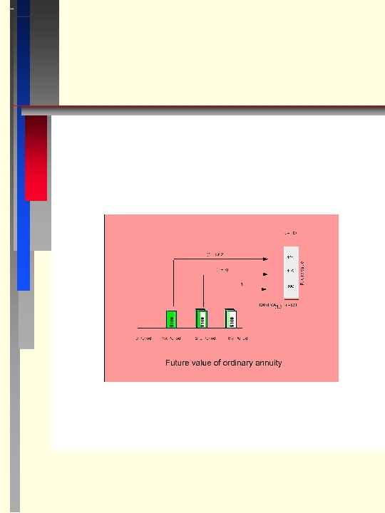
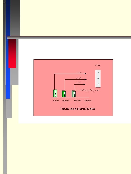
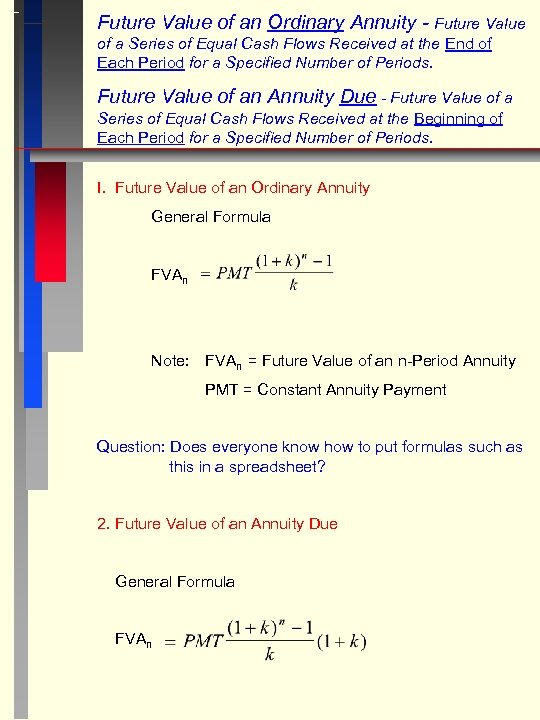 Future Value of an Ordinary Annuity - Future Value of a Series of Equal Cash Flows Received at the End of Each Period for a Specified Number of Periods. Future Value of an Annuity Due - Future Value of a Series of Equal Cash Flows Received at the Beginning of Each Period for a Specified Number of Periods. I. Future Value of an Ordinary Annuity General Formula FVAn Note: FVAn = Future Value of an n-Period Annuity PMT = Constant Annuity Payment Question: Does everyone know how to put formulas such as this in a spreadsheet? 2. Future Value of an Annuity Due General Formula FVAn
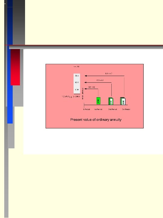
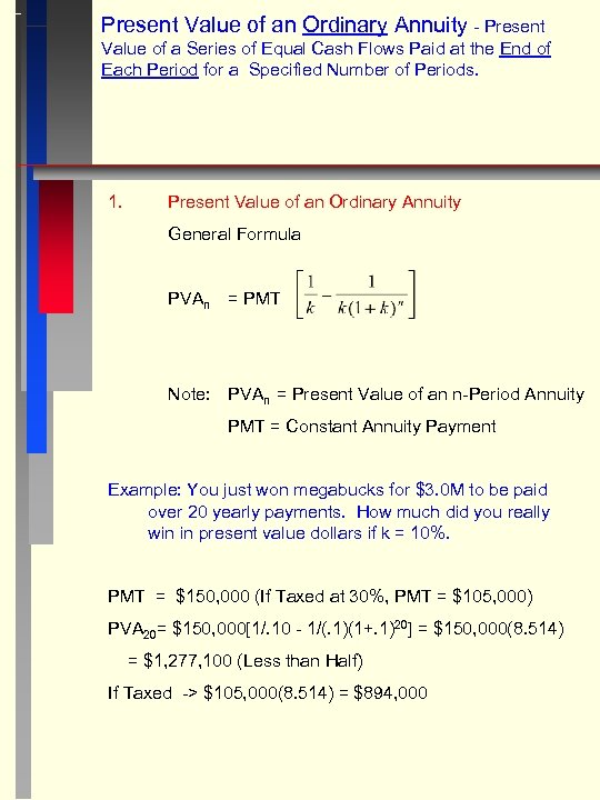 Present Value of an Ordinary Annuity - Present Value of a Series of Equal Cash Flows Paid at the End of Each Period for a Specified Number of Periods. 1. Present Value of an Ordinary Annuity General Formula PVAn = PMT Note: PVAn = Present Value of an n-Period Annuity PMT = Constant Annuity Payment Example: You just won megabucks for $3. 0 M to be paid over 20 yearly payments. How much did you really win in present value dollars if k = 10%. PMT = $150, 000 (If Taxed at 30%, PMT = $105, 000) PVA 20= $150, 000[1/. 10 - 1/(. 1)(1+. 1)20] = $150, 000(8. 514) = $1, 277, 100 (Less than Half) If Taxed -> $105, 000(8. 514) = $894, 000
 2. Note: For the Present Value of an Annuity Due, just multiply the above by (1 + k) because the money is earning interest for one additional year. For an Infinite Annuity (n = ∞) the formula above reduces to PVA = PMT [1/k] = PMT/k Example: Redo the Lottery example except assume that you receive payments for ever. PVA = $150, 000/. 10 = $1, 500, 000 This is not much more than a receiving payments for only 20 years because payments after 20 years are not worth much - discounted heavily. Note: The infinite annuity is often a good approximation to a long annuity and is easy to calculate. 3. All of these valuation equations are additive, meaning that you can get the value of a complex series of cash flows by recognizing that a complex cash flow is made up of simpler cash flows, value each simple cash flow and add to get the complex cash flow value.
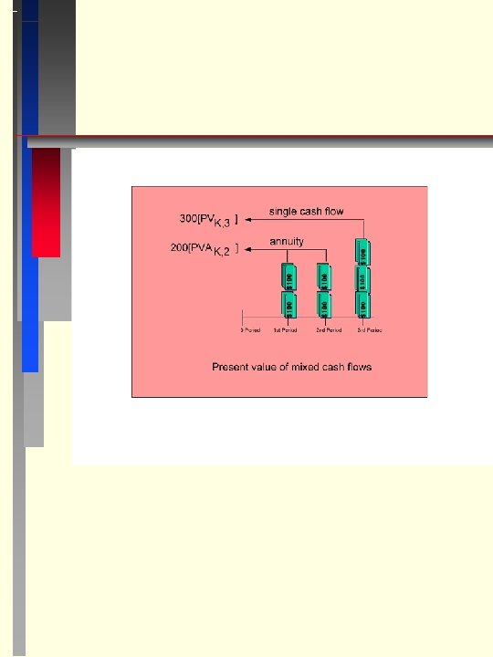
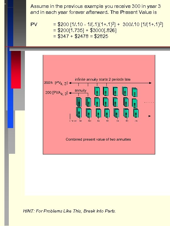 Assume in the previous example you receive 300 in year 3 and in each year forever afterward. The Present Value is PV = $200 [1/. 10 - 1/(. 1)(1+. 1)2] + 300/. 10 [1/(1+. 1)2] = $200[1. 735] + $3000[. 826] = $347 + $2478 = $2825 HINT: For Problems Like This, Break Into Parts.
 Effective vs. Nominal Interest Rates “The Effective Rate is the True Rate of Interest per Year and the Nominal Rate is the Quoted Rate per Year” 3. Effective vs. Nominal keff = (1+knom/m)m - 1 If interest is compounded “m” times annually, we must adjust k and n in the formulas above, to take account of the additional interest earned during a year. Example: A nominal rate of 16% is compounded quarterly. Thus, each quarter we earn 4% on the money in the account. k 4 = k/m = 16%/4 = 4% keff = (1+knom/m)m - 1 = (1+. 16/4)4 -1 =. 1698 => 17% (Effective Rate) Therefore, although the nominal rate is 16%, we effectively earn about 17%.
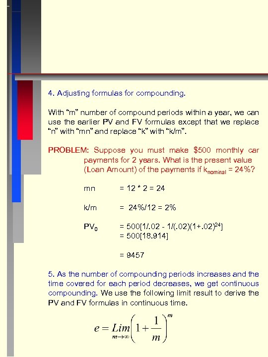 4. Adjusting formulas for compounding. With “m” number of compound periods within a year, we can use the earlier PV and FV formulas except that we replace “n” with “mn” and replace “k” with “k/m”. PROBLEM: Suppose you must make $500 monthly car payments for 2 years. What is the present value (Loan Amount) of the payments if knominal = 24%? mn = 12 * 2 = 24 k/m = 24%/12 = 2% PV 0 = 500[1/. 02 - 1/(. 02)(1+. 02)24] = 500[18. 914] = 9457 5. As the number of compounding periods increases and the time covered for each period decreases, we get continuous compounding. We use the following limit result to derive the PV and FV formulas in continuous time.
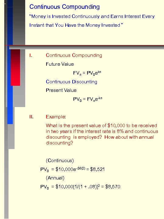 Continuous Compounding “Money is Invested Continuously and Earns Interest Every Instant that You Have the Money Invested ” I. Continuous Compounding Future Value FVn = PV 0 ekn Continuous Discounting Present Value PV 0 = FVne-kn II. Example: What is the present value of $10, 000 to be received in two years if the interest rate is 8% and continuous discounting is employed? How about with annual discounting? (Continuous) PV 0 = $10, 000 e-. 08(2) = $8, 521 (Annual) PV 0 = $10, 000[1/(1 +. 08)]2 = $8, 570
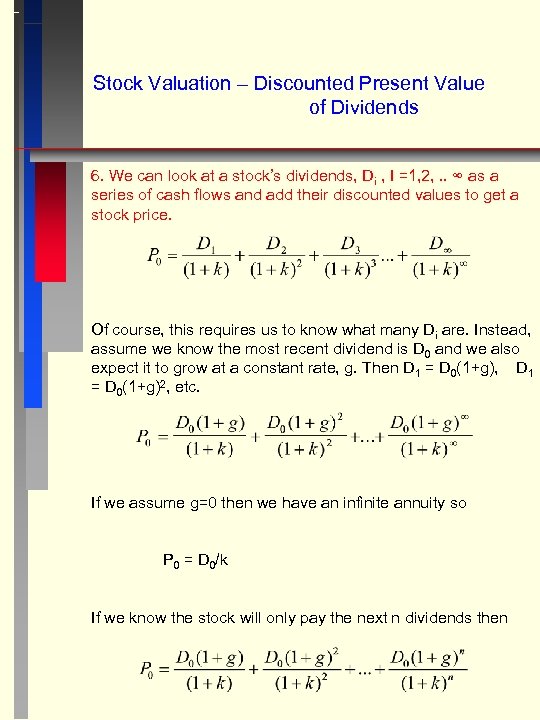 Stock Valuation – Discounted Present Value of Dividends 6. We can look at a stock’s dividends, Di , I =1, 2, . . ∞ as a series of cash flows and add their discounted values to get a stock price. Of course, this requires us to know what many Di are. Instead, assume we know the most recent dividend is D 0 and we also expect it to grow at a constant rate, g. Then D 1 = D 0(1+g), D 1 = D 0(1+g)2, etc. If we assume g=0 then we have an infinite annuity so P 0 = D 0/k If we know the stock will only pay the next n dividends then
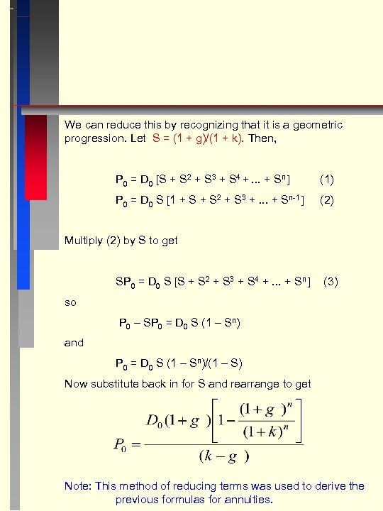 We can reduce this by recognizing that it is a geometric progression. Let S = (1 + g)/(1 + k). Then, P 0 = D 0 [S + S 2 + S 3 + S 4 +. . . + Sn ] (1) P 0 = D 0 S [1 + S 2 + S 3 +. . . + Sn-1 ] (2) Multiply (2) by S to get SP 0 = D 0 S [S + S 2 + S 3 + S 4 +. . . + Sn ] (3) so P 0 – SP 0 = D 0 S (1 – Sn) and P 0 = D 0 S (1 – Sn)/(1 – S) Now substitute back in for S and rearrange to get Note: This method of reducing terms was used to derive the previous formulas for annuities.
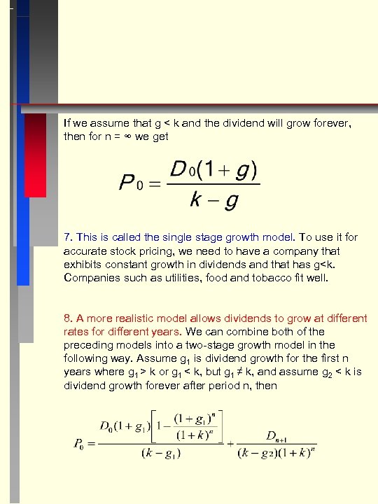 If we assume that g < k and the dividend will grow forever, then for n = ∞ we get 7. This is called the single stage growth model. To use it for accurate stock pricing, we need to have a company that exhibits constant growth in dividends and that has g
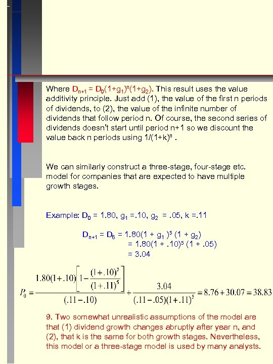 Where Dn+1 = D 0(1+g 1)n(1+g 2). This result uses the value additivity principle. Just add (1), the value of the first n periods of dividends, to (2), the value of the infinite number of dividends that follow period n. Of course, the second series of dividends doesn’t start until period n+1 so we discount the value back n periods using 1/(1+k)n. We can similarly construct a three-stage, four-stage etc. model for companies that are expected to have multiple growth stages. Example: D 0 = 1. 80, g 1 =. 10, g 2 =. 05, k =. 11 Dn+1 = D 6 = 1. 80(1 + g 1 )5 (1 + g 2) = 1. 80(1 +. 10)5 (1 +. 05) = 3. 04 9. Two somewhat unrealistic assumptions of the model are that (1) dividend growth changes abruptly after year n, and (2), that k is the same for both growth stages. Nevertheless, this model or a three-stage model is used by many analysts.
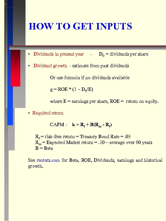 HOW TO GET INPUTS • Dividends in present year - D 0 = dividends per share • Dividend growth - estimate from past dividends Or use formula if no dividends available g = ROE * (1 – D 0/E) where E = earnings per share, ROE = return on equity. • Required return CAPM - k = Rf + B(Rm - Rf) Rf = risk-free return = Treasury Bond Rate =. 03 Rm = Expected Market return =. 10 – average over 60 years B = Beta See reuters. com for Beta, ROE, Dividends, earnings and historical growth.
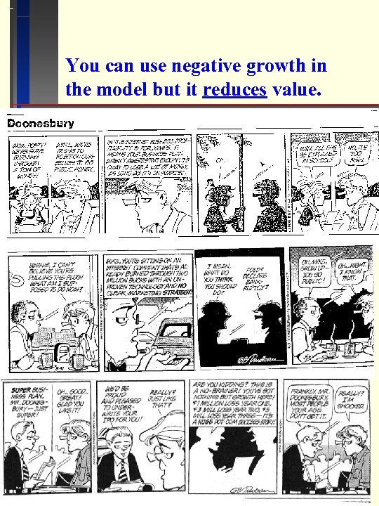 You can use negative growth in the model but it reduces value.
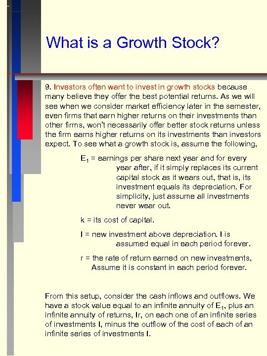 What is a Growth Stock? 9. Investors often want to invest in growth stocks because many believe they offer the best potential returns. As we will see when we consider market efficiency later in the semester, even firms that earn higher returns on their investments than other firms, won’t necessarily offer better stock returns unless the firm earns higher returns on its investments than investors expect. To see what a growth stock is, assume the following, E 1 = earnings per share next year and for every year after, if it simply replaces its current capital stock as it wears out, that is, its investment equals its depreciation. For simplicity, just assume all investments never wear out. k = its cost of capital. I = new investment above depreciation. I is assumed equal in each period forever. r = the rate of return earned on new investments, Assume it is constant in each period forever. From this setup, consider the cash inflows and outflows. We have a stock value equal to an infinite annuity of E 1, plus an infinite annuity of returns, Ir, on each one of an infinite series of investments I, minus the outflow of the cost of each of an infinite series of investments I.
![So Where [Ir/k] is the present value of all of the returns from one So Where [Ir/k] is the present value of all of the returns from one](https://present5.com/presentation/57aadcf35dfcb4aefb43f9900f56f385/image-23.jpg) So Where [Ir/k] is the present value of all of the returns from one year’s new investment. Now the value of an infinite series of these investments equals [Ir/k]/k so that, And rearranging this gives, The first term is the value of a no-growth firm, one that only replaces its current capital stock. The second term defines what we mean by a growth stock (r > k) or a declining stock (r < k). This depends upon whether a firm’s new investments earn more or less than its cost of capital.
So Where [Ir/k] is the present value of all of the returns from one year’s new investment. Now the value of an infinite series of these investments equals [Ir/k]/k so that, And rearranging this gives, The first term is the value of a no-growth firm, one that only replaces its current capital stock. The second term defines what we mean by a growth stock (r > k) or a declining stock (r < k). This depends upon whether a firm’s new investments earn more or less than its cost of capital.
![10. The term [r – k] is just the result of an Internal Rate 10. The term [r – k] is just the result of an Internal Rate](https://present5.com/presentation/57aadcf35dfcb4aefb43f9900f56f385/image-24.jpg) 10. The term [r – k] is just the result of an Internal Rate of Return rule that says that the firm should invest in all projects that earn a return greater than its cost of capital. If it has no such projects, it should not invest and should not grow. This became an issue for some internet firms that had raised lots of cash in 1999 and early 2000. It was clear by mid-2000 that further investments in their businesses would earn them less than their costs of capital. Nevertheless, they continued to make investments. Question: Given the equation above, what do you think happened to their stock prices? Question: Why do you think they kept investing anyway? (illustrates importance of agency/behavioral theory - Shanta) 11. This model, or a similar but more complex model, is used to calculate the present value of growth opportunities (PVGO). The PVGO is just the second term. More often than not, r is difficult to observe, but P 0, E 1 and k are observable, so that PVGO is calculated as PVGO = P 0 – E 1/k This approach can be used to find how the market values brand names, patents etc. , which offer high returns for future investments. It is the market’s valuation because we use P 0 and assume that the price is set correctly by the market.
10. The term [r – k] is just the result of an Internal Rate of Return rule that says that the firm should invest in all projects that earn a return greater than its cost of capital. If it has no such projects, it should not invest and should not grow. This became an issue for some internet firms that had raised lots of cash in 1999 and early 2000. It was clear by mid-2000 that further investments in their businesses would earn them less than their costs of capital. Nevertheless, they continued to make investments. Question: Given the equation above, what do you think happened to their stock prices? Question: Why do you think they kept investing anyway? (illustrates importance of agency/behavioral theory - Shanta) 11. This model, or a similar but more complex model, is used to calculate the present value of growth opportunities (PVGO). The PVGO is just the second term. More often than not, r is difficult to observe, but P 0, E 1 and k are observable, so that PVGO is calculated as PVGO = P 0 – E 1/k This approach can be used to find how the market values brand names, patents etc. , which offer high returns for future investments. It is the market’s valuation because we use P 0 and assume that the price is set correctly by the market.
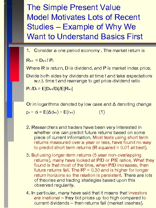 The Simple Present Value Model Motivates Lots of Recent Studies – Example of Why We Want to Understand Basics First 1. Consider a one period economy. The market return is Rt+1 = Dt+1 / Pt Where R is return, D is dividend, and P is market index price. Divide both sides by dividends at time t and take expectations w. r. t. time t and rearrange to get price-dividend ratio Pt /Dt = E[Dt+1/Dt]/E[Rt+1] Or in logarithms denoted by low case and Δ denoting change pt − dt = E(Δdt+1) − E(rt+1) (1) 2. Researchers and traders have been very interested in whether one can predict future returns based on some piece of current information. Most tests using short term returns measured over a year or less, have found no way to predict short term returns (R-squared = 0. 01 at best). 3. But using longer-term returns (5 year non-overlapping returns), many have looked at P/D or P/E ratios. What they found is that most of the time, when P/D increases, then future returns fall. The R 2 = 0. 30 and is higher for longer return horizons so the relation is persistent. There are lots of theories and trading strategies based upon this observed regularity. 4. In particular, many have said that it means that investors are irrational – they bid prices up too high compared to current dividends – then returns fall (market crashes).
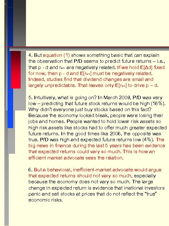 4. But equation (1) shows something basic that can explain the observation that P/D seems to predict future returns – i. e. , that p - d and rt+1 are negatively related. If we hold E[Δd] fixed for now, then p - d and E[rt+1] must be negatively related. Indeed, studies find that dividend changes are small and largely unpredictable. That leaves only E[rt+1] to drive p – d. 5. Intuitively, what is going on? In March 2009, P/D was very low – predicting that future stock returns would be high (16%). Why didn’t everyone just buy stocks based on this fact? Because the economy looked bleak, people were losing their jobs and homes. People wanted to hold lower risk assets so high risk assets like stocks had to offer much greater expected future returns. In the good times like 2006, the opposite was true. P/D was high and expected future returns low (4%). The big news in finance during the last 5 years has been evidence that expected returns could vary so much. This is how an efficient market advocate sees the relation. 6. But a behavioral, inefficient-market advocate would argue that expected returns should not vary so much, especially because the economy does not vary so much. The large change in expected return is evidence that irrational investors panic and sell stocks at prices that do not reflect the “true” economic risks.
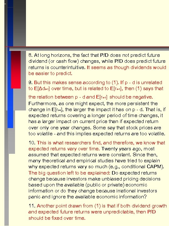 8. At long horizons, the fact that P/D does not predict future dividend (or cash flow) changes, while P/D does predict future returns is counterintuitive. It seems as though dividends would be easier to predict. 9. But this makes sense according to (1). If p - d is unrelated to E[Δdt+1] over time, but is related to E[rt+1], then (1) says that the relation between p - d and E[rt+1] should be negative. Furthermore, as one might expect, the more persistent the change in E[rt+t], the larger the impact it has on p - d. That is, if expected returns covering a longer period of time changes, it has a larger impact on current price than if expected return over only one year changes. Some say that stock prices are too volatile - and this implies expected returns are too volatile. 10. This is what researchers find, and therefore, we know that expected returns vary over time. Twenty years ago, most assumed that expected returns were constant. Since then, many theoretical and empirical studies have tried to explain why expected returns vary so much (e. g. , conditional CAPM). The big question left to be explained: Do expected returns change because investors make unbiased pricing decisions based upon the available (public or private) economic information or do they change because irrational investors panic and ignore the available economic information? 11. Another point drawn from (1) is that if both dividend growth and expected future returns were unpredictable, then P/D should be fixed over time.
 Implications and Extensions 1. Cost of capital for firms varies over time. 2. The CAPM with fixed expected returns is wrong. 3. Beta risk reflects variation between a firm’s expected returns (not cash flows) and the market’s expected returns. These can change over different horizons. So betas can change over different horizons. 4. The whole analysis can be applied to other variables that predict returns besides P/D, or those variables can be analyzed along with P/D. Examples include bond yield spread, consumption/wealth, investment/capital, share issuance, book/market, size, lagged returns, etc. 5. The analysis can also explain the behavior of other assets. For example, for bonds, the slope of the term structure (spread between short and long bonds) can be explained by changes in expected returns rather than changes in interest rates (coupons). And foreign exchange holdings, the spread between long and short futures prices can be predicted by changes in expected returns rather than differences in domestic and foreign interest rates. This explains why often the high interest rate currency appreciates over time rather than depreciates, as would be expected from the simple foreign exchange futures model. That model assumes risk is fixed (e. g. zero) over time but changing risk and expected returns could drive the result.
 Four Methods of Asset Pricing 1. Discounting expected cash flows using a risk-adjusted discount rate - Pro - most common – traditional approach - Con - requires a model to estimate risk-adjustment 2. Discount risk-adjusted expected cash flows by the risk free rate - Pro – risk-free rate is known – LIBOR, not Tbonds - Con – need to estimate the expected cash flow insurance premium (risk-adjustment) – swaps, futures spreads, insurance 3. Modify the objective probabilities to get the risk-neutral probabilities, calculate expected cash flows based on them, and discount at the risk-free rate. - Pro - avoids assumption on utility function or equilibrium - Con - requires a replicating portfolio and return distribution assumptions. 4. Decompose cash flows into Arrow-Debreau state specific elements and sum. - Pro – no distribution or utility function assumptions - Con - Need the states and state specific security prices – see prediction markets – intrade. com


