1e1f3c4d11ab7e41fb9ff4b717ec14e5.ppt
- Количество слайдов: 52
Lecture 1 BSB 370 Managing Quality and Operations
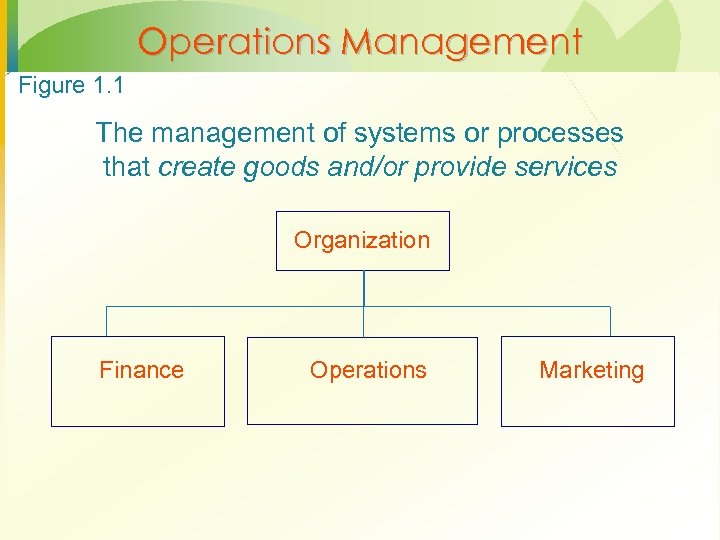
Operations Management Figure 1. 1 The management of systems or processes that create goods and/or provide services Organization Finance Operations Marketing
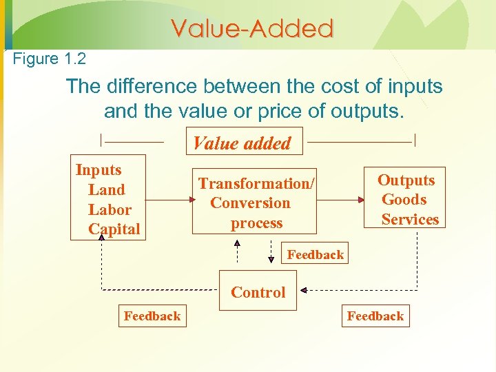
Value-Added Figure 1. 2 The difference between the cost of inputs and the value or price of outputs. Value added Inputs Land Labor Capital Transformation/ Conversion process Outputs Goods Services Feedback Control Feedback
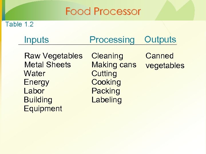
Food Processor Table 1. 2 Inputs Processing Outputs Raw Vegetables Metal Sheets Water Energy Labor Building Equipment Cleaning Making cans Cutting Cooking Packing Labeling Canned vegetables
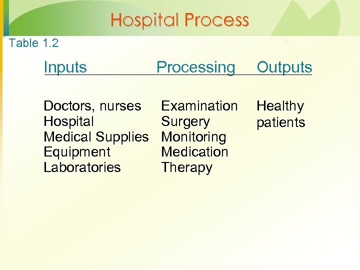
Hospital Process Table 1. 2 Inputs Doctors, nurses Hospital Medical Supplies Equipment Laboratories Processing Outputs Examination Surgery Monitoring Medication Therapy Healthy patients
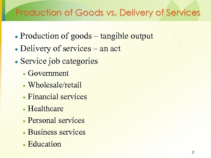
Production of Goods vs. Delivery of Services Production of goods – tangible output · Delivery of services – an act · Service job categories · Government · Wholesale/retail · Financial services · Healthcare · Personal services · Business services · Education · 6
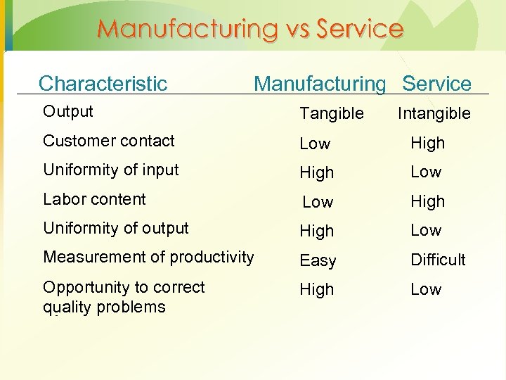
Manufacturing vs Service Characteristic Manufacturing Service Output Tangible Customer contact Low High Uniformity of input High Low Labor content Low High Uniformity of output High Low Measurement of productivity Easy Difficult Opportunity to correct quality problems High Low High Intangible
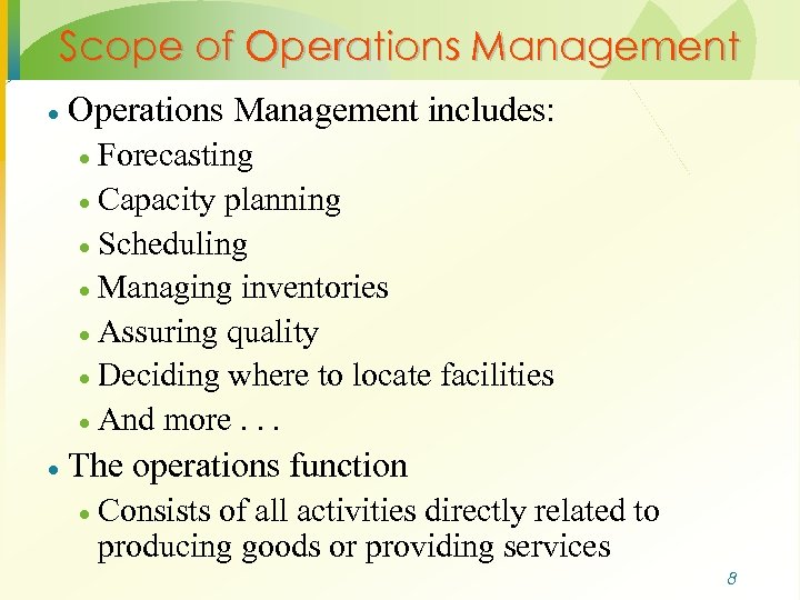
Scope of Operations Management · Operations Management includes: Forecasting · Capacity planning · Scheduling · Managing inventories · Assuring quality · Deciding where to locate facilities · And more. . . · · The operations function · Consists of all activities directly related to producing goods or providing services 8
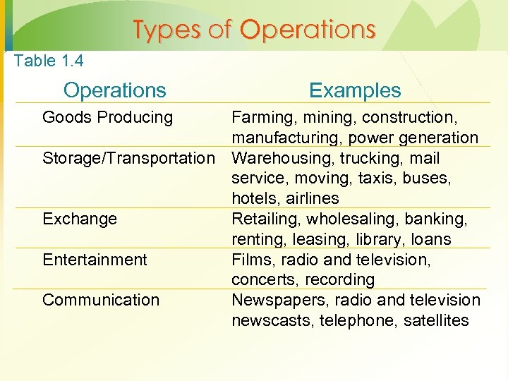
Types of Operations Table 1. 4 Operations Goods Producing Examples Farming, mining, construction, manufacturing, power generation Storage/Transportation Warehousing, trucking, mail service, moving, taxis, buses, hotels, airlines Exchange Retailing, wholesaling, banking, renting, leasing, library, loans Entertainment Films, radio and television, concerts, recording Communication Newspapers, radio and television newscasts, telephone, satellites
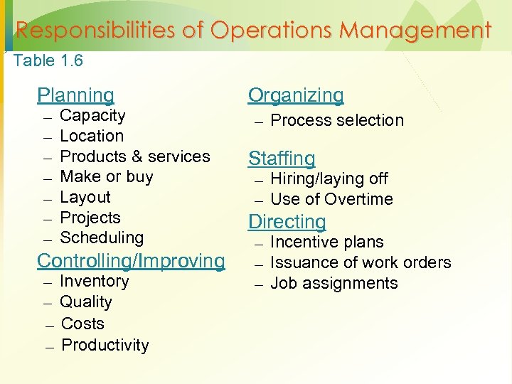
Responsibilities of Operations Management Table 1. 6 Planning – – – – Capacity Location Products & services Make or buy Layout Projects Scheduling Controlling/Improving – – Inventory Quality Costs Productivity Organizing – Process selection Staffing – Hiring/laying off – Use of Overtime Directing – Incentive plans – Issuance of work orders – Job assignments
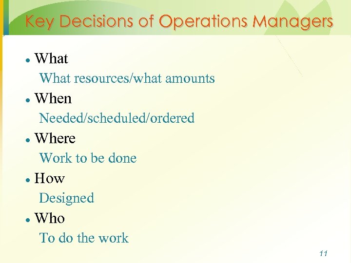
Key Decisions of Operations Managers · What resources/what amounts · When Needed/scheduled/ordered · Where Work to be done · How Designed · Who To do the work 11
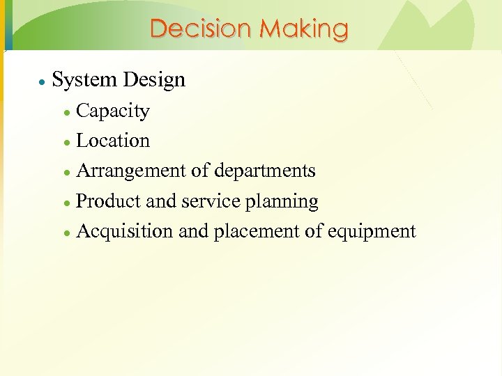
Decision Making · System Design Capacity · Location · Arrangement of departments · Product and service planning · Acquisition and placement of equipment ·
Decision Making · System Operation Management of personnel · Inventory planning and control · Scheduling · Project Management · Quality assurance ·
Decision Making Models · Quantitative approaches · Analysis of trade-offs · 14
Models A model is an abstraction of reality. – Physical – Schematic – Mathematical Tradeoffs What are the pros and cons of models?
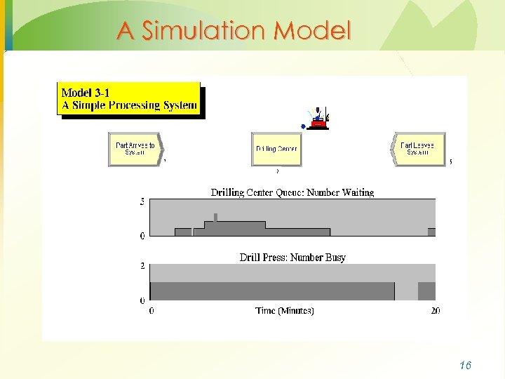
A Simulation Model 16
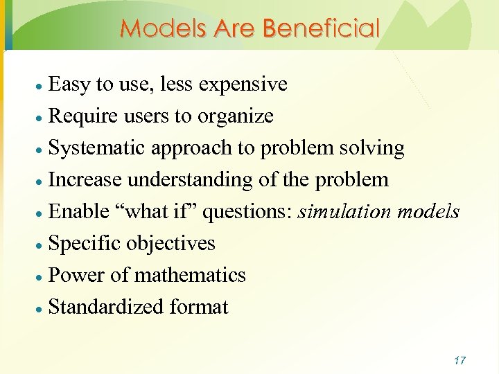
Models Are Beneficial Easy to use, less expensive · Require users to organize · Systematic approach to problem solving · Increase understanding of the problem · Enable “what if” questions: simulation models · Specific objectives · Power of mathematics · Standardized format · 17
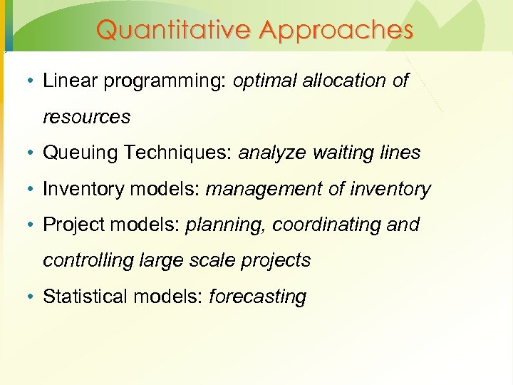
Quantitative Approaches • Linear programming: optimal allocation of resources • Queuing Techniques: analyze waiting lines • Inventory models: management of inventory • Project models: planning, coordinating and controlling large scale projects • Statistical models: forecasting
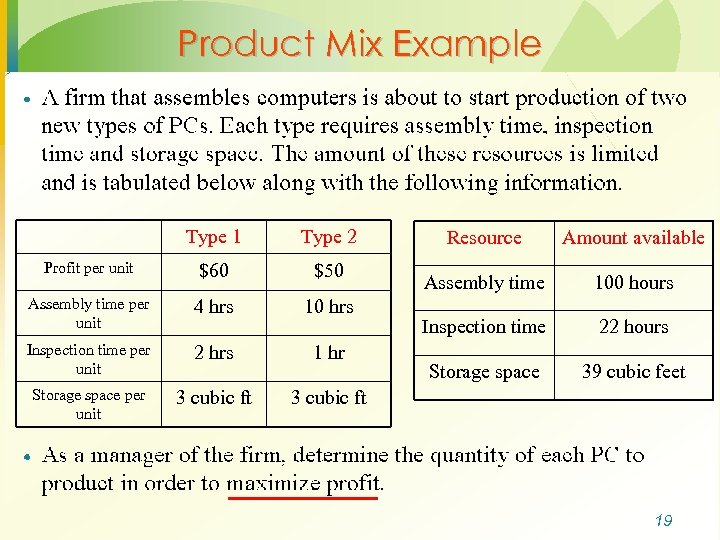
Product Mix Example Type 1 Type 2 Profit per unit $60 $50 Assembly time per unit 4 hrs 10 hrs Inspection time per unit 2 hrs 1 hr Storage space per unit 3 cubic ft Resource Amount available Assembly time 100 hours Inspection time 22 hours Storage space 39 cubic feet 19
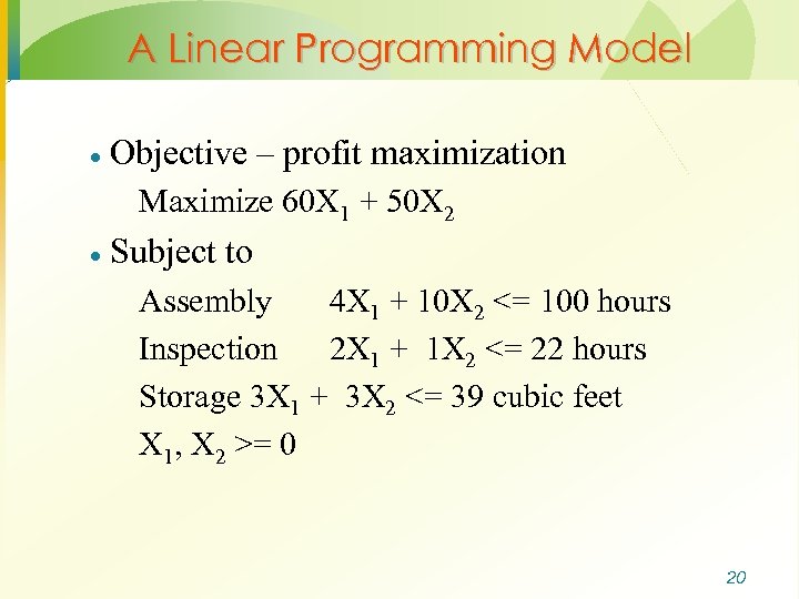
A Linear Programming Model · Objective – profit maximization Maximize 60 X 1 + 50 X 2 · Subject to Assembly 4 X 1 + 10 X 2 <= 100 hours Inspection 2 X 1 + 1 X 2 <= 22 hours Storage 3 X 1 + 3 X 2 <= 39 cubic feet X 1, X 2 >= 0 20
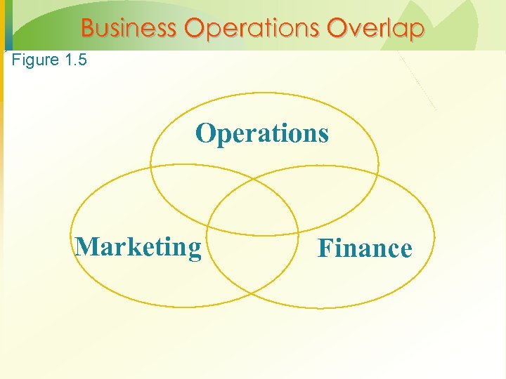
Business Operations Overlap Figure 1. 5 Operations Marketing Finance
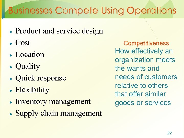
Businesses Compete Using Operations · · · · Product and service design Cost Location Quality Quick response Flexibility Inventory management Supply chain management Competitiveness How effectively an organization meets the wants and needs of customers relative to others that offer similar goods or services 22
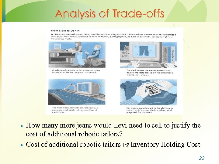
Analysis of Trade-offs · · How many more jeans would Levi need to sell to justify the cost of additional robotic tailors? Cost of additional robotic tailors vs Inventory Holding Cost 23
Competitiveness, Strategy, and Productivity Chapter 2 24
Productivity · Productivity A measure of the effective use of resources · Usually expressed as the ratio of output to input · · Productivity ratios are used for Planning workforce requirements · Scheduling equipment · Financial analysis · 25
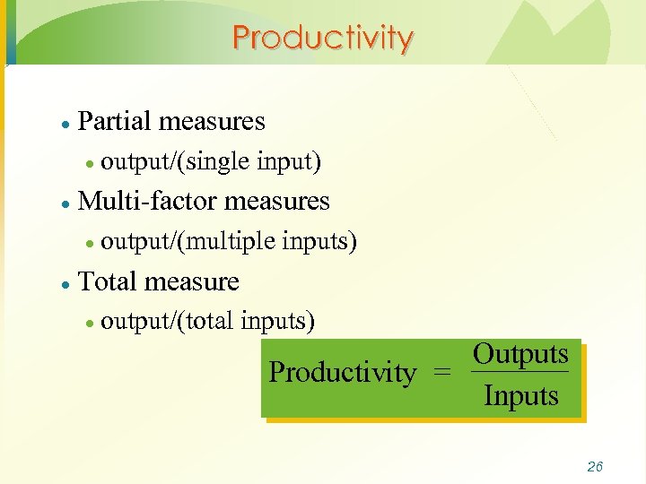
Productivity · Partial measures · output/(single · input) Multi-factor measures · output/(multiple · inputs) Total measure · output/(total inputs) Outputs Productivity = Inputs 26
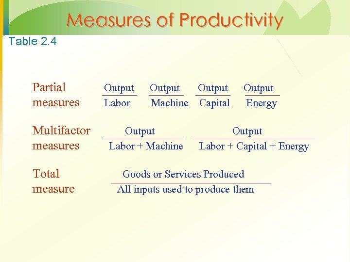
Measures of Productivity Table 2. 4 Partial measures Multifactor measures Total measure Output Labor Output Machine Capital Output Labor + Machine Output Energy Output Labor + Capital + Energy Goods or Services Produced All inputs used to produce them
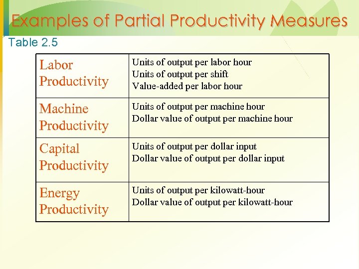
Examples of Partial Productivity Measures Table 2. 5 Labor Productivity Units of output per labor hour Units of output per shift Value-added per labor hour Machine Productivity Units of output per machine hour Dollar value of output per machine hour Capital Productivity Units of output per dollar input Dollar value of output per dollar input Energy Productivity Units of output per kilowatt-hour Dollar value of output per kilowatt-hour
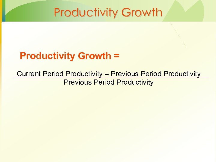
Productivity Growth = Current Period Productivity – Previous Period Productivity
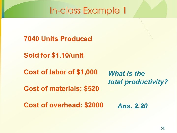
In-class Example 1 7040 Units Produced Sold for $1. 10/unit Cost of labor of $1, 000 Cost of materials: $520 Cost of overhead: $2000 What is the total productivity? Ans. 2. 20 30
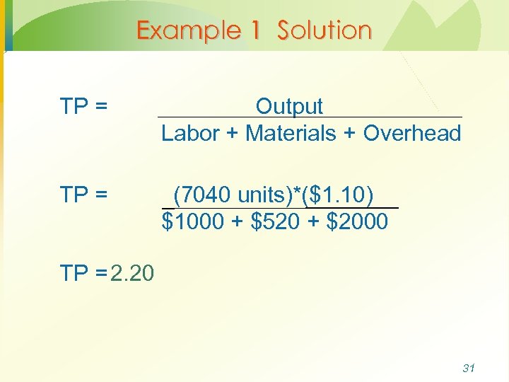
Example 1 Solution TP = Output Labor + Materials + Overhead TP = (7040 units)*($1. 10) $1000 + $520 + $2000 TP = 2. 20 31
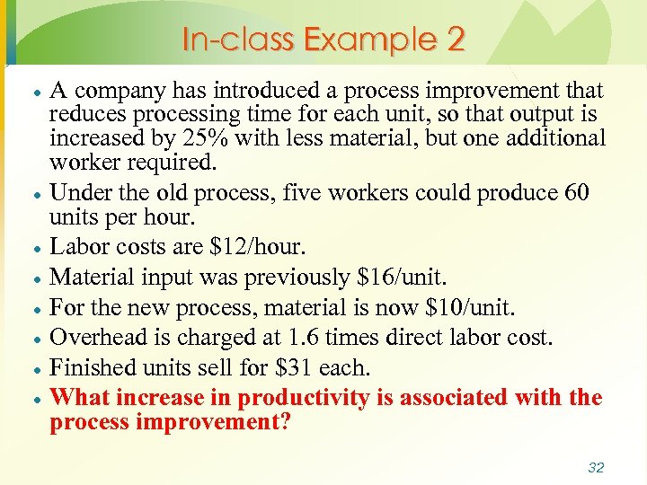
In-class Example 2 · · · · A company has introduced a process improvement that reduces processing time for each unit, so that output is increased by 25% with less material, but one additional worker required. Under the old process, five workers could produce 60 units per hour. Labor costs are $12/hour. Material input was previously $16/unit. For the new process, material is now $10/unit. Overhead is charged at 1. 6 times direct labor cost. Finished units sell for $31 each. What increase in productivity is associated with the process improvement? 32
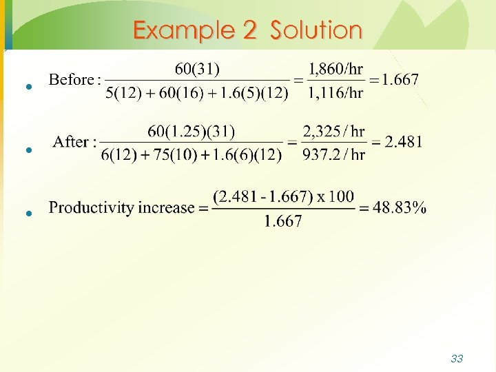
Example 2 Solution · · · 33
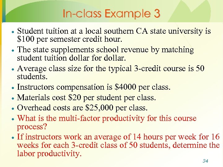
In-class Example 3 · · · · Student tuition at a local southern CA state university is $100 per semester credit hour. The state supplements school revenue by matching student tuition dollar for dollar. Average class size for the typical 3 -credit course is 50 students. Instructors compensation is $4000 per class. Materials cost $20 per student per class. Overhead costs are $25, 000 per class. What is the multi-factor productivity for this course process? If instructors work an average of 14 hours per week for 16 weeks for each 3 -credit class of 50 students, determine the labor productivity. 34
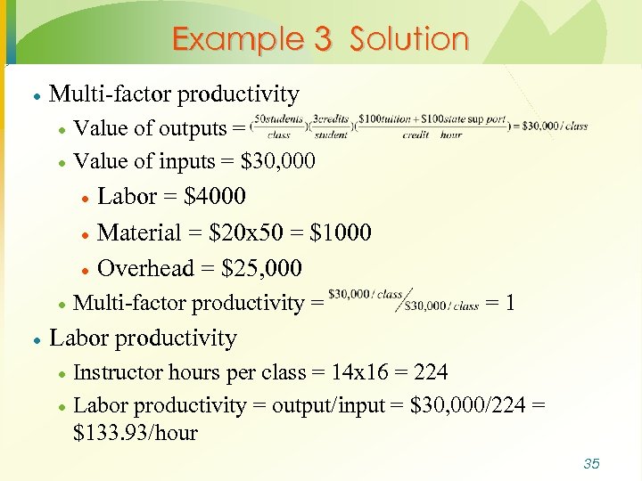
Example 3 Solution · Multi-factor productivity · · Value of outputs = Value of inputs = $30, 000 · · · Labor = $4000 Material = $20 x 50 = $1000 Overhead = $25, 000 Multi-factor productivity = =1 Labor productivity · · Instructor hours per class = 14 x 16 = 224 Labor productivity = output/input = $30, 000/224 = $133. 93/hour 35
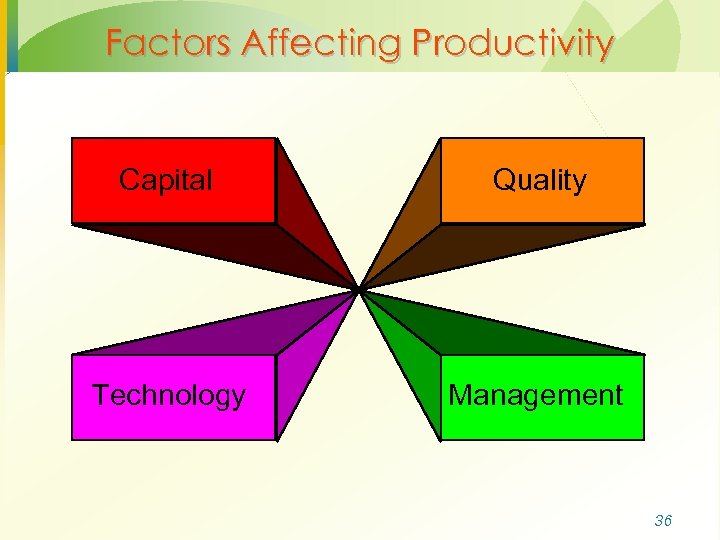
Factors Affecting Productivity Capital Quality Technology Management 36
Other Factors Affecting Productivity Standardization · Quality · Use of Internet · Computer viruses · Searching for lost or misplaced items · Scrap rates · New workers · Bottleneck operations · 37
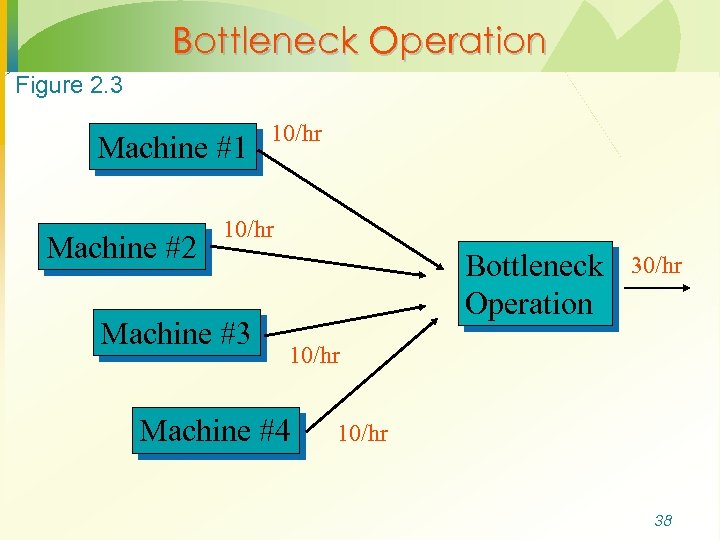
Bottleneck Operation Figure 2. 3 Machine #1 Machine #2 10/hr Machine #3 Bottleneck Operation 30/hr 10/hr Machine #4 10/hr 38
Cost, Revenue, Profit Models & Break-even Analysis Chapter 5
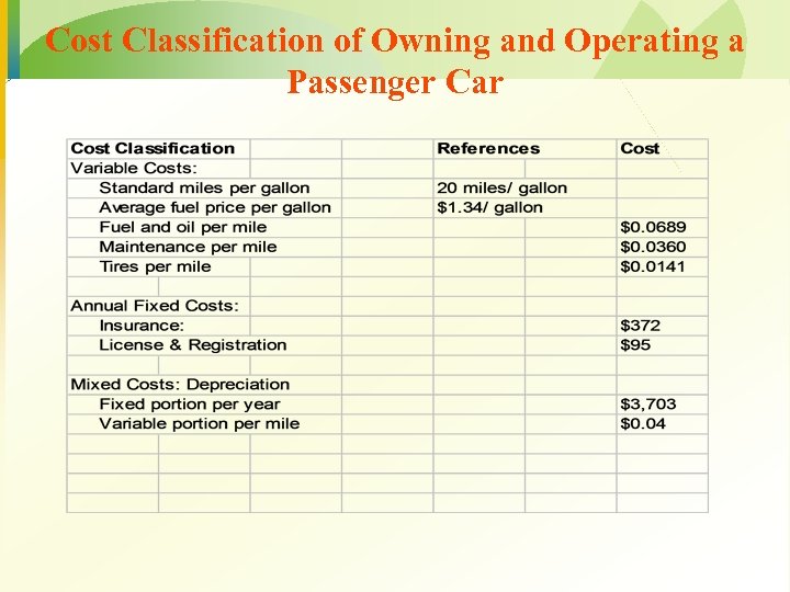
Cost Classification of Owning and Operating a Passenger Car
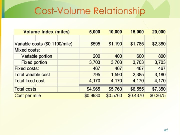
Cost-Volume Relationship 41
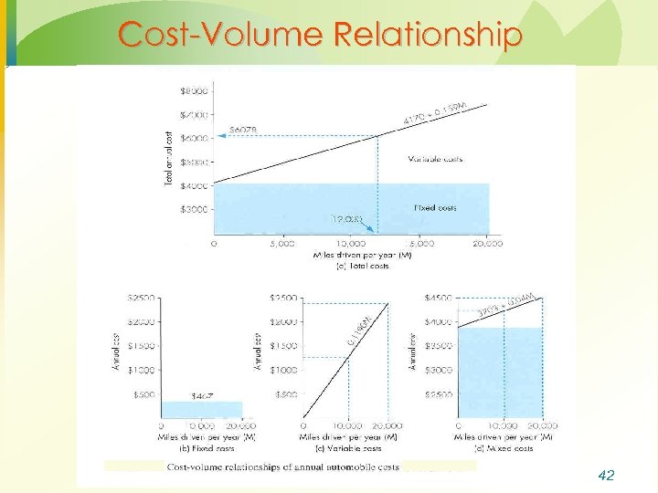
Cost-Volume Relationship 42
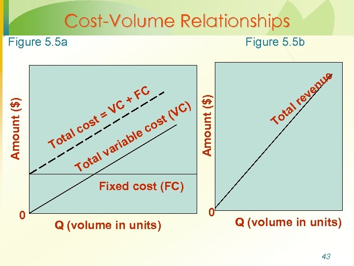
Cost-Volume Relationships Figure 5. 5 b lc ota T st o VC = ota T C) t (V s co e bl ia r a lv FC + Amount ($) Figure 5. 5 a ue en v re l a ot T Fixed cost (FC) 0 Q (volume in units) 43
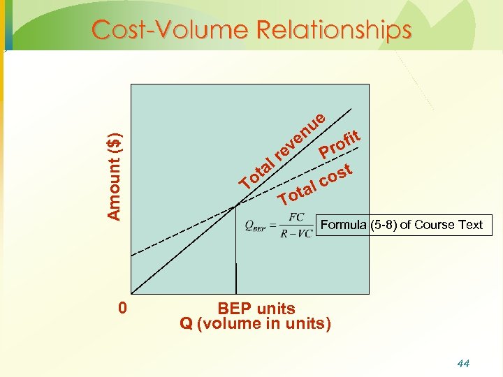
Amount ($) Cost-Volume Relationships 0 ve ta o T ue n re l fit ro P t os al c ot T Formula (5 -8) of Course Text BEP units Q (volume in units) 44
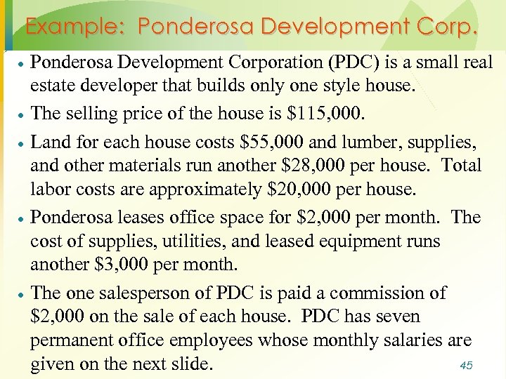
Example: Ponderosa Development Corp. · · · Ponderosa Development Corporation (PDC) is a small real estate developer that builds only one style house. The selling price of the house is $115, 000. Land for each house costs $55, 000 and lumber, supplies, and other materials run another $28, 000 per house. Total labor costs are approximately $20, 000 per house. Ponderosa leases office space for $2, 000 per month. The cost of supplies, utilities, and leased equipment runs another $3, 000 per month. The one salesperson of PDC is paid a commission of $2, 000 on the sale of each house. PDC has seven permanent office employees whose monthly salaries are 45 given on the next slide.
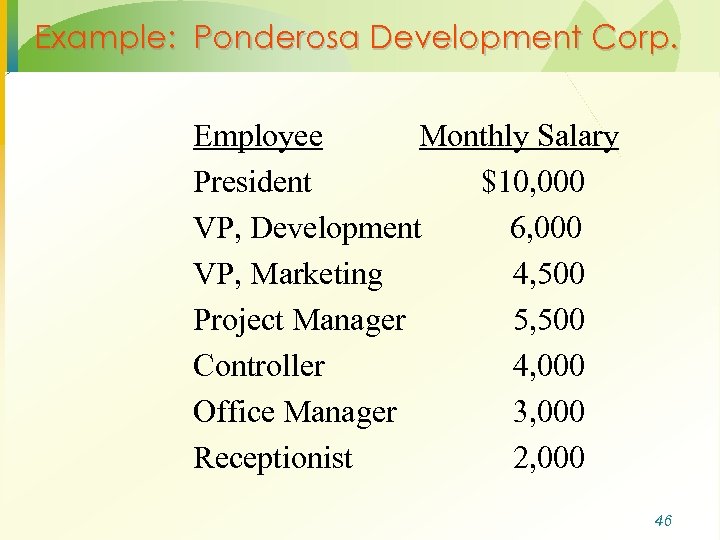
Example: Ponderosa Development Corp. Employee Monthly Salary President $10, 000 VP, Development 6, 000 VP, Marketing 4, 500 Project Manager 5, 500 Controller 4, 000 Office Manager 3, 000 Receptionist 2, 000 46
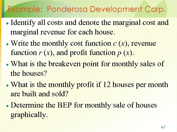
Example: Ponderosa Development Corp. Identify all costs and denote the marginal cost and marginal revenue for each house. · Write the monthly cost function c (x), revenue function r (x), and profit function p (x). · What is the breakeven point for monthly sales of the houses? · What is the monthly profit if 12 houses per month are built and sold? · Determine the BEP for monthly sale of houses graphically. · 47
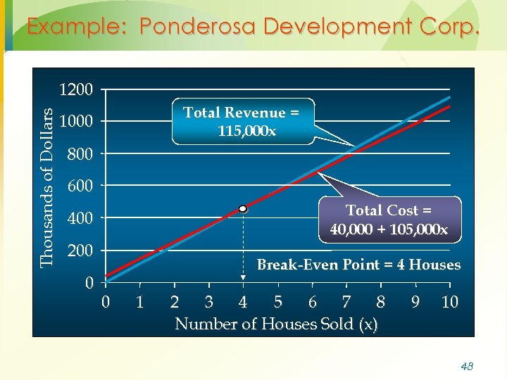
Example: Ponderosa Development Corp. Thousands of Dollars 1200 Total Revenue = 115, 000 x 1000 800 600 Total Cost = 40, 000 + 105, 000 x 400 200 0 Break-Even Point = 4 Houses 0 1 2 3 4 5 6 7 8 Number of Houses Sold (x) 9 10 48
Influence Chart Price Quantity Sold Total Revenue Variable Cost Unit Cost Profit Total Cost Fixed Cost
Example: Step Fixed Costs A manager has the option of purchasing 1, 2 or 3 machines · Fixed costs and potential volumes are as follows: · # of machines 1 2 3 Total annual FC ($) 9600 15000 20000 Range of output 0 – 300 301 – 600 601 – 900 Variable cost = $10/unit and revenue = $40/unit · If the projected annual demand is between 580 and 630 units, how many machines should the manager purchase? · 50
Break-Even Problem with Step Fixed Costs Figure 5. 6 a & b combined Total Cost C T C= +V FC Total Revenue + FC C =T C V BEVs 3 machines C =T C F +V C 2 machines 1 machine Quantity Step fixed costs and variable costs. 51
Assumptions of Cost-Volume Analysis 1. 2. 3. 4. 5. 6. One product is involved Everything produced can be sold Variable cost per unit is the same regardless of volume Fixed costs do not change with volume Revenue per unit constant with volume Revenue per unit exceeds variable cost per unit 52
1e1f3c4d11ab7e41fb9ff4b717ec14e5.ppt