Lecture 1 BNFO 601 Usman Roshan Course

Lecture 1 BNFO 601 Usman Roshan

Course overview • Perl progamming language (and some Unix basics) – Unix basics – Intro Perl exercises – Dynamic programming and Viterbi algorithm in Perl • Sequence analysis – Algorithms for exact and heuristic pairwise alignment – Hidden Markov models – BLAST – Short read alignments – Whole genome sequence alignment – High performance methods for very large datasets

Overview (contd) • Grade: Two 25% exams, 30% final exam, and six programming assignments (20%) • Exams will cover Perl and bioinformatics algorithms • Recommended Texts: – Introduction to Bioinformatics Algorithms by Pavel Pevzner and Neil Jones – Biological sequence analysis by Durbin et. al. – Introduction to Bioinformatics by Arthur Lesk – Beginning Perl for Bioinformatics by James Tisdall – Introduction to Machine Learning by Ethem Alpaydin

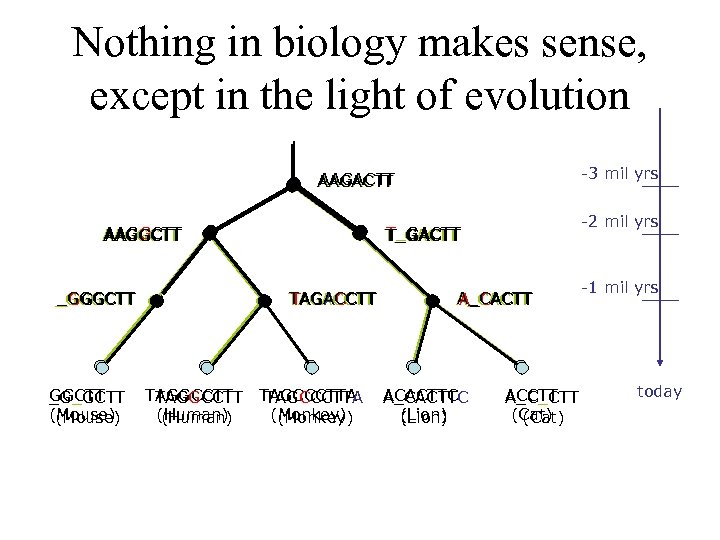
Nothing in biology makes sense, except in the light of evolution -3 mil yrs AAGACTT AAGGCTT _GGGCTT _G_GCTT (Mouse) TAGACCTT TAGGCCTT (Human) -2 mil yrs T_GACTT TAGCCCTTA (Monkey) A_CACTT ACACTTC A_CACTTC (Lion) ACCTT A_C_CTT (Cat) -1 mil yrs today

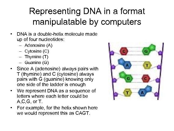
Representing DNA in a format manipulatable by computers • DNA is a double-helix molecule made up of four nucleotides: – – Adenosine (A) Cytosine (C) Thymine (T) Guanine (G) • Since A (adenosine) always pairs with T (thymine) and C (cytosine) always pairs with G (guanine) knowing only one side of the ladder is enough • We represent DNA as a sequence of letters where each letter could be A, C, G, or T. • For example, for the helix shown here we would represent this as CAGT.

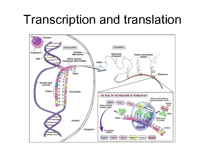
Transcription and translation

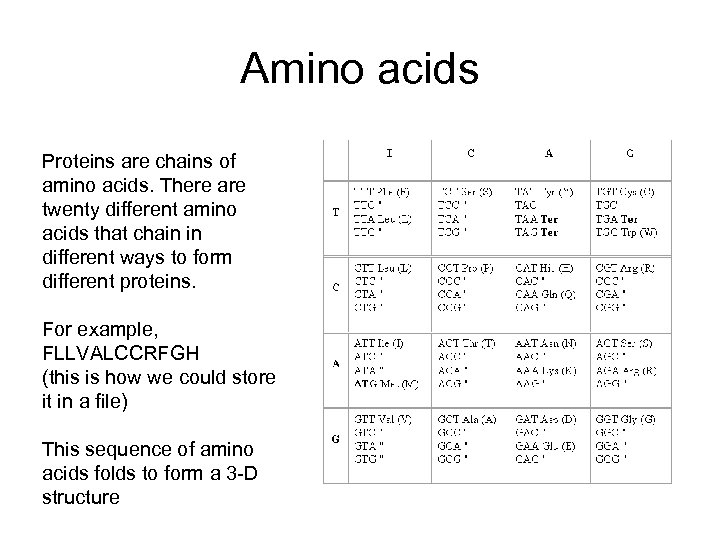
Amino acids Proteins are chains of amino acids. There are twenty different amino acids that chain in different ways to form different proteins. For example, FLLVALCCRFGH (this is how we could store it in a file) This sequence of amino acids folds to form a 3 -D structure

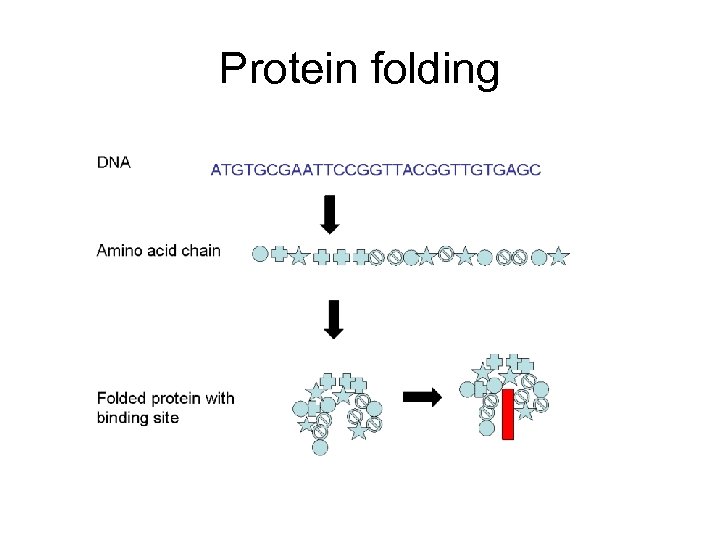
Protein folding

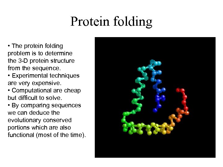
Protein folding • The protein folding problem is to determine the 3 -D protein structure from the sequence. • Experimental techniques are very expensive. • Computational are cheap but difficult to solve. • By comparing sequences we can deduce the evolutionary conserved portions which are also functional (most of the time).

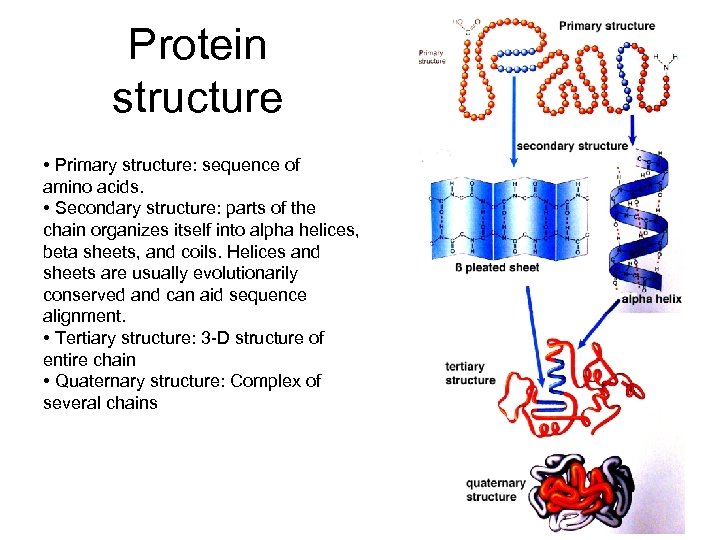
Protein structure • Primary structure: sequence of amino acids. • Secondary structure: parts of the chain organizes itself into alpha helices, beta sheets, and coils. Helices and sheets are usually evolutionarily conserved and can aid sequence alignment. • Tertiary structure: 3 -D structure of entire chain • Quaternary structure: Complex of several chains

Key points • DNA can be represented as strings consisting of four letters: A, C, G, and T. They could be very long, e. g. thousands and even millions of letters • Proteins are also represented as strings of 20 letters (each letter is an amino acid). Their 3 -D structure determines the function to a large extent.

Comparison of sequences • Fundamental in bioinformatics • Many applications – Evolutionary conserved regions – Functional sites in proteins – Phylogeny reconstruction – Protein structural contact prediction – Gene splicing – Genome assembly – Database search

Pairwise sequence alignment • Comparison of two sequences • We want to determine the substitutions, insertions, and deletions that occurred between the two sequences

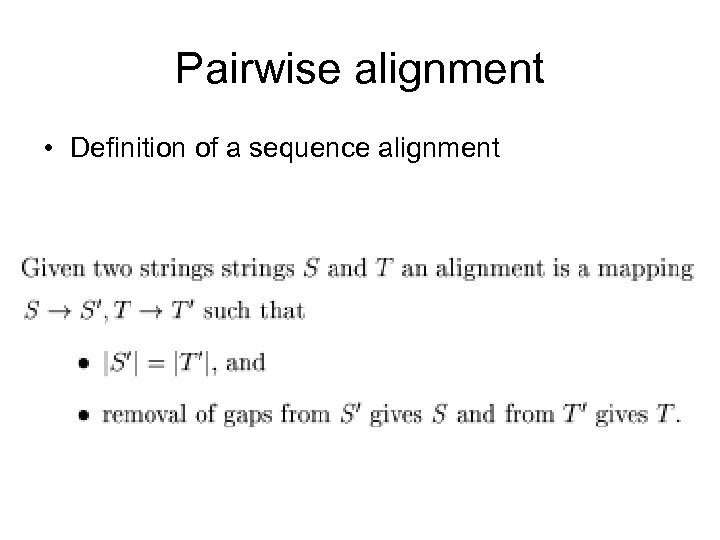
Pairwise alignment • Definition of a sequence alignment

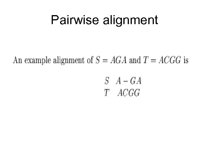
Pairwise alignment

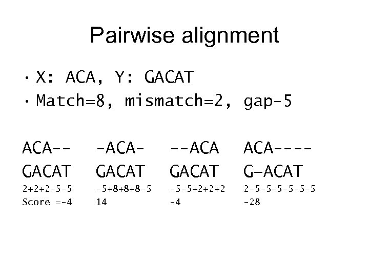
Pairwise alignment • X: ACA, Y: GACAT • Match=8, mismatch=2, gap-5 ACA-GACAT -ACAGACAT --ACA GACAT ACA---G—ACAT 2+2+2 -5 -5 Score =-4 -5+8+8+8 -5 14 -5 -5+2+2+2 -4 2 -5 -5 -5 -28

Traceback • We can compute an alignment of DNA (or protein or RNA) sequences X and Y with a traceback matrix T. • Sequence X is aligned along the rows and Y along the columns. • Each entry of the matrix T contains D, L, or U specifying diagonal, left or upper

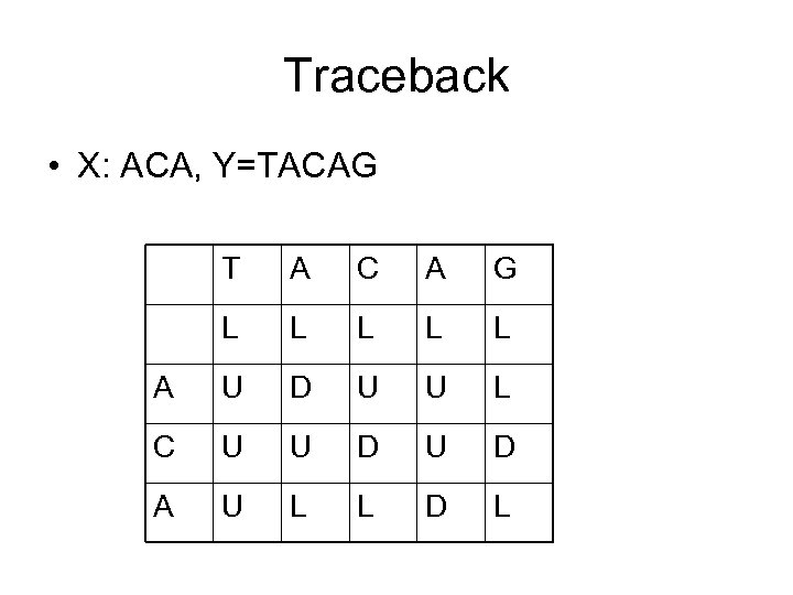
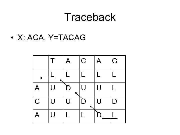
Traceback • X: ACA, Y=TACAG T A C A G L L L A U D U U L C U U D A U L L D L

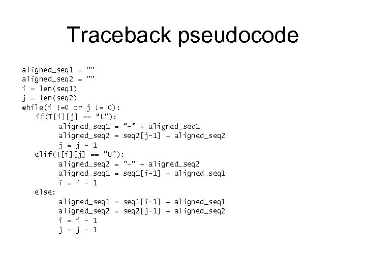
Traceback pseudocode aligned_seq 1 = "" aligned_seq 2 = "" i = len(seq 1) j = len(seq 2) while(i !=0 or j != 0): if(T[i][j] == “L”): aligned_seq 1 = “-” + aligned_seq 1 aligned_seq 2 = seq 2[j-1] + aligned_seq 2 j = j - 1 elif(T[i][j] == "U"): aligned_seq 2 = "-" + aligned_seq 2 aligned_seq 1 = seq 1[i-1] + aligned_seq 1 i = i - 1 else: aligned_seq 1 = seq 1[i-1] + aligned_seq 1 aligned_seq 2 = seq 2[j-1] + aligned_seq 2 i = i - 1 j = j - 1

Optimal alignment • An alignment can be specified by the traceback matrix. • How do we determine the traceback for the highest scoring alignment? • Needleman-Wunsch algorithm for global alignment – First proposed in 1970 – Widely used in genomics/bioinformatics – Dynamic programming algorithm

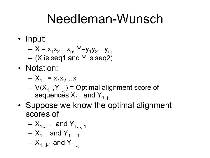
Needleman-Wunsch • Input: – X = x 1 x 2…xn, Y=y 1 y 2…ym – (X is seq 1 and Y is seq 2) • Notation: – X 1. . i = x 1 x 2…xi – V(X 1. . i, Y 1. . j) = Optimal alignment score of sequences X 1. . i and Y 1. . j. • Suppose we know the optimal alignment scores of – X 1…i-1 and Y 1…j-1 – X 1…i and Y 1. . . j-1 – X 1. . . i-1 and Y 1…j

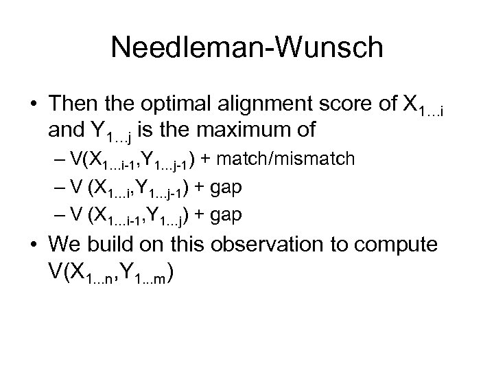
Needleman-Wunsch • Then the optimal alignment score of X 1…i and Y 1…j is the maximum of – V(X 1…i-1, Y 1…j-1) + match/mismatch – V (X 1…i, Y 1…j-1) + gap – V (X 1…i-1, Y 1…j) + gap • We build on this observation to compute V(X 1. . . n, Y 1. . . m)

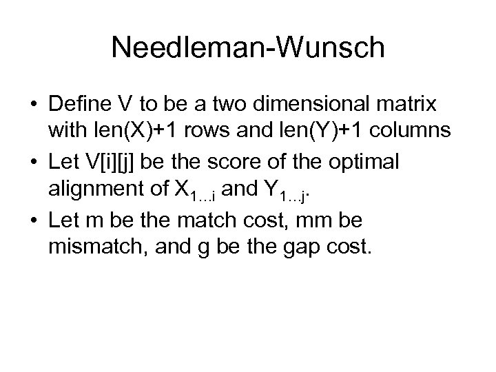
Needleman-Wunsch • Define V to be a two dimensional matrix with len(X)+1 rows and len(Y)+1 columns • Let V[i][j] be the score of the optimal alignment of X 1…i and Y 1…j. • Let m be the match cost, mm be mismatch, and g be the gap cost.

NW pseudocode Initialization: for i = 1 to length of seq 1 { V[i][0] = i*g; } For i = 1 to length of seq 2 { V[0][i] = i*g; } Recurrence: for i = 1 to length of seq 1{ for j = 1 to length of seq 2{ V[i][j] = max { V[i-1][j-1] + m(or mm) V[i-1][j] + g V[i][j-1] + g if(maximum is V[i-1][j-1] + m(or mm)) then T[i][j] = ‘D’ else if (maximum is V[i-1][j] + g) then T[i][j] = ‘U’ else then T[i][j] = ‘L’ } }

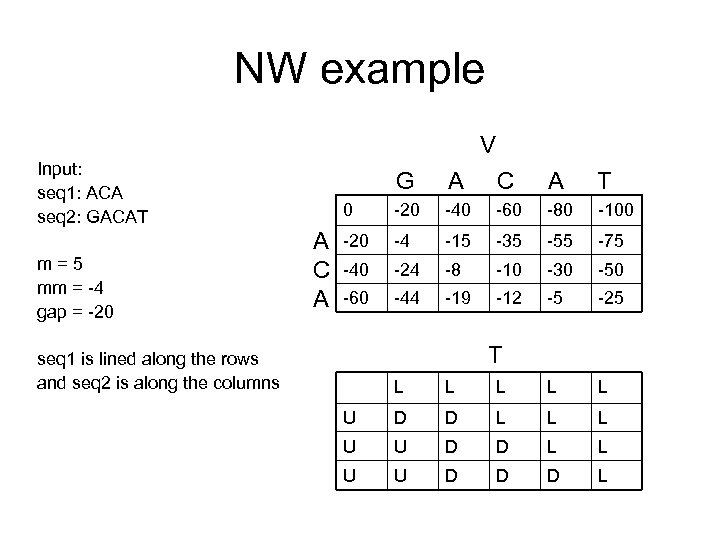
NW example V Input: seq 1: ACA seq 2: GACAT m=5 mm = -4 gap = -20 G C A T 0 A C A A -20 -40 -60 -80 -100 -20 -4 -15 -35 -55 -75 -40 -24 -8 -10 -30 -50 -60 -44 -19 -12 -5 -25 T seq 1 is lined along the rows and seq 2 is along the columns L L L U D D L L L U U D D D L

NW parameters • How do we pick gap penalty and match/mismatch costs? • Proteins/RNA both have 3 -D structure. • We can produce high quality manual alignments by hand if the structure is available. • These alignments can then serve as a benchmark to train gap parameters so that the alignment program produces correct alignments.

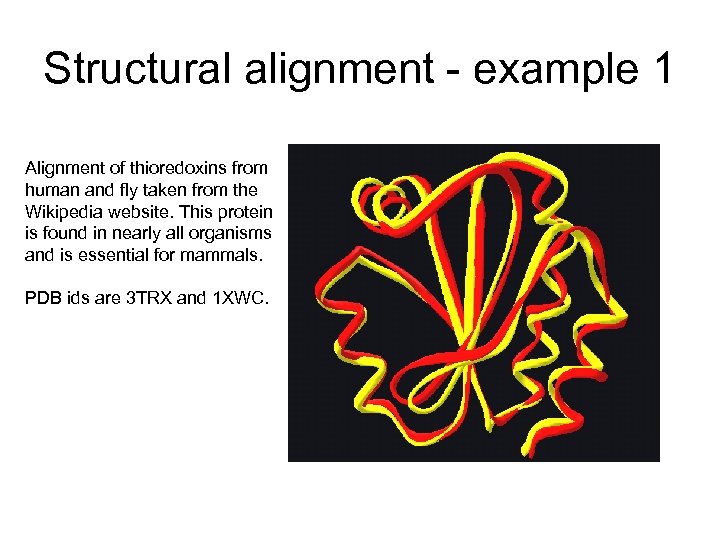
Structural alignment - example 1 Alignment of thioredoxins from human and fly taken from the Wikipedia website. This protein is found in nearly all organisms and is essential for mammals. PDB ids are 3 TRX and 1 XWC.

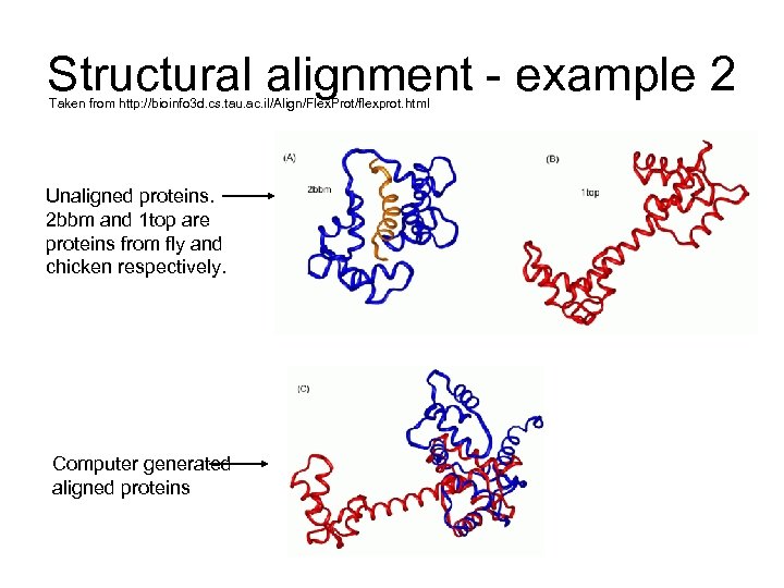
Structural alignment - example 2 Taken from http: //bioinfo 3 d. cs. tau. ac. il/Align/Flex. Prot/flexprot. html Unaligned proteins. 2 bbm and 1 top are proteins from fly and chicken respectively. Computer generated aligned proteins

Benchmark alignments • Protein alignment benchmarks – BAli. BASE, SABMARK, PREFAB, HOMSTRAD are frequently used in studies for protein alignment. – Proteins benchmarks are generally large and have been in the research community for sometime now. – BAli. BASE 3. 0

NW parameters • With a procedure called cross-validation we use the benchmark to train gap parameters so that the alignment program produces correct alignments. • How can we quantify the “correctness” of a test alignment with respect to a reference? • We measure the number of pairs in the test that are also aligned in the reference alignment. • This is also called the sum-of-pairs accuracy.

NW parameters • For match and mismatch costs we use a more direct approach: log likelihood scores • We calculate probabilities from the benchmark • The same cannot be done for gap penalties because in benchmarks because of uncertainties in gap placements

Biologically realistic scoring matrices • PAM and BLOSUM are most popular • PAM was developed by Margaret Dayhoff and co-workers in 1978 by examining 1572 mutations between 71 families of closely related proteins • BLOSUM is more recent and computed from blocks of sequences with sufficient similarity

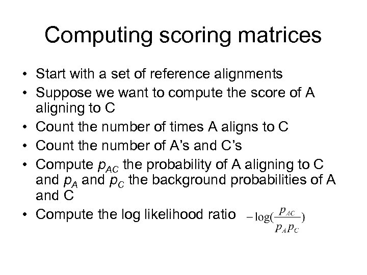
Computing scoring matrices • Start with a set of reference alignments • Suppose we want to compute the score of A aligning to C • Count the number of times A aligns to C • Count the number of A’s and C’s • Compute p. AC the probability of A aligning to C and p. A and p. C the background probabilities of A and C • Compute the log likelihood ratio

Next week • Basics of Unix • Perl programming – Basics – Exercises – Dynamic programming solution to sequence alignment in Perl